
Full Outlook Report
Summary
Thank you to the groups that contributed to the 2015 June report; 32 contributions (one of which is regional only) is a record for the Sea Ice Outlook! We also welcome several new groups this year.
This June Outlook report was developed by lead authors, Cecilia Bitz (UW), Ed Blanchard-Wrigglesworth (UW), and Jim Overland (NOAA), with contributions from the rest of the SIPN leadership team, and with a section analyzing the model contributions by François Massonnet, Université catholique de Louvain and Catalan Institute of Climate Sciences.
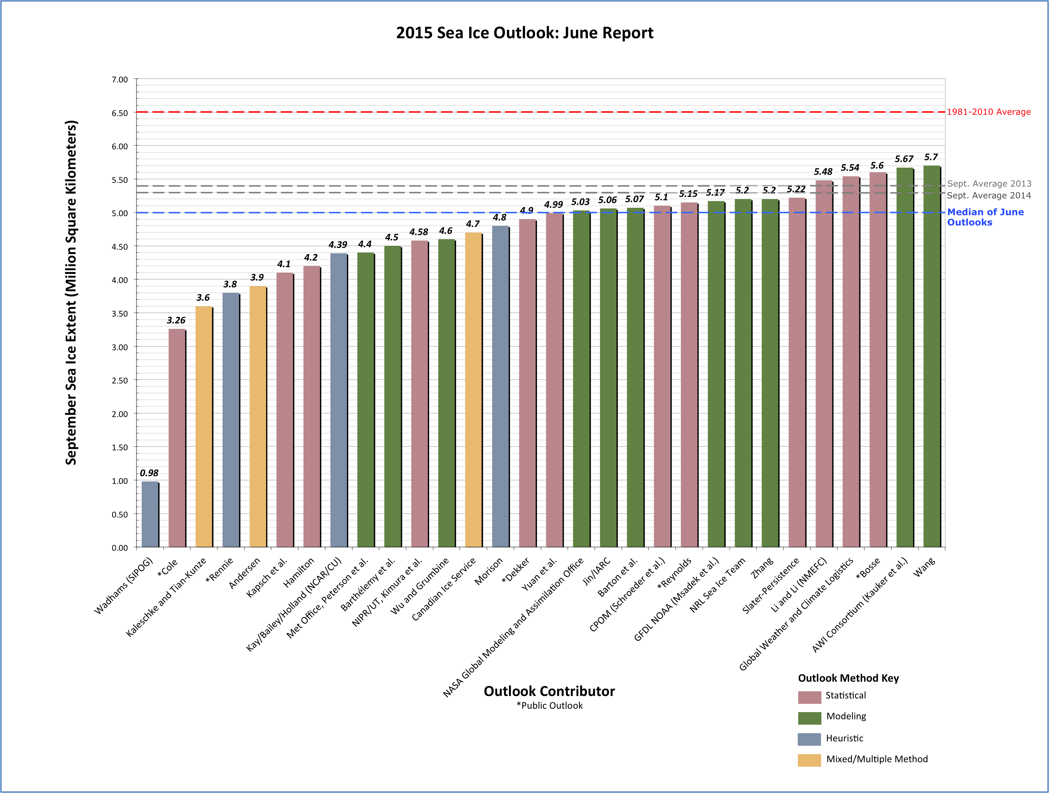
The median Outlook value for September 2015 sea ice extent is 5.0 million square kilometers with quartiles of 4.4 and 5.2 million square kilometers (See Figure 1 in the full report, below). Contributions are based on a range of methods: statistical, numerical models, estimates based on trends, and subjective information. We have a large spread in the Outlook contributions, which is not surprising given the wide-ranging observed values for the September extent in the past few years. The overall range (excluding an extreme outlier) is 3.3 to 5.7 million square kilometers. The median Outlook value is up from 4.7 million square kilometers in 2014. These values compare to observed values of 4.3 million square kilometers in 2007, 4.6 million square kilometers in 2011, 3.6 million square kilometers in 2012 and 5.3 million square kilometers in 2014.
A discussion of 11 dynamical model contributions shows that the variance among the individual outlooks is substantially less than last year and as a whole, dynamic models predict a larger September sea ice extent with less spread than for 2014. A section on regional predictions includes discussion on predictions for sea ice probability (SIP), showing that higher SIP is predicted in 2015 than in 2014 in the Beaufort and East Greenland seas, while smaller SIP is predicted along the East Siberian and Kara Seas. Finally, a section on current conditions includes discussion of this spring’s rate of decline of ice extent, a comparison of sea ice thickness products, and atmospheric conditions.
Overview
The Outlook contributions this June are based on a range of methods: statistical, dynamical models, estimates based on trends, and subjective information. We value the diversity of contributions. While we have a record number of Outlook contributions this month, the width of the distribution of Outlooks has narrowed compared to last year: The interquartile spread across all types of contributions is 0.8 million square kilometers, which is a decrease by 0.1 million square kilometers since last year. The overall range is still quite large: Excluding an extreme outlier, the range is 3.3 to 5.7 million square kilometers. The forecasted range is slightly wider than the observed range of September sea ice extent during the history of the Outlook, which is 3.6 million square kilometers in 2012 to 5.4 million square kilometers in 2009.
Over the years since the SIO started, we have seen a shift from less quantitative heuristic methods towards more quantitative contributions based on statistical and dynamical models. This month, we had 12 contributions using statistical methods and 11 using dynamic models. Despite an increase in number, the distribution of Outlooks for each of these types compared to last year has stayed about the same among statistical methods but narrowed among dynamical models (see next section for more information about the models).
 for September 2015 sea ice extent. We do not show submissions that were received late, thus n=30 in this figure and all subsequent figures.")
Download a high-resolution version of Figure 1.

Comment On Dynamical Modeling Contributions
Provided by François Massonnet, Université catholique de Louvain, Belgium, & Catalan Institute of Climate Sciences, Spain
2015 Modeling Contributions at a Glance
This year, we received 11 contributions from dynamical modeling groups. Six of them were obtained from integration of fully coupled general circulation models (in blue on Figure 3), and five from ocean-sea ice models forced by atmospheric reanalysis or other atmospheric model output (in green on Figure 3). The median extent predicted by these 11 models is 5.07 million km2 (mean: 5.05 million km2), which is higher than last year's prediction for the June report (4.65 and 4.71 million km2, respectively).
Ten of the 11 modeling contributions include a statement of uncertainty. Uncertainty is reported in Figure 3 using error bars. Uncertainties were in all cases obtained from ensemble runs (from 7 to 42 members) intended to sample atmospheric variability only. Note that a coordinated sensitivity experiment to initial conditions is currently running in parallel to the regular Sea Ice Outlook activities, and will be reported on elsewhere.
Decomposition of the Spread in the 2015 Model Predictions
The variance among individual model outlooks (the dots in Figure 3) amounts to (0.41 million km2) 2, which is substantially less than last year (0.73 million km2)2. Assuming that the number of ensemble members used to produce the individual submissions is large enough, each outlook averages away the unpredictable noise due to the atmosphere. In other words, the standard deviation of 0.41 million km2 captures the uncertainty associated with factors that can (hopefully) be controlled and reduced in the future: initial conditions, resolution, and model errors. The remainder of total spread is associated with the unpredictable, chaotic evolution of the atmosphere between June and September. We estimate that this variance due to chaos amounts to (0.45 million km2)2.
How we estimated the spread due to chaos.
In other words, about half of the 2015 prediction uncertainty is due to irreducible errors while the other half is directly related to spread in model configurations and initial conditions. This leaves room for improvement in the design of forecasting systems. Last year, irreducible errors were far exceeded by controllable errors, likely due to the presence of one rather high contribution.
In summary, as a whole, dynamic models predict a larger September sea ice extent with less spread than for 2014. Note however that, in 2014, model predictions issued in June underestimated the actual September 2014 sea ice extent by about 0.6 million km2.
 and from all other methods (grey). The dots are the outlook themselves and the intervals are the uncertainty ranges provided by the groups. Definitions of uncertainty were left to the discretion of the groups themselves, and should therefore be compared with caution. The middle dashed horizontal line is the median of the outlooks from dynamical modeling groups. The lower (upper) dashed horizontal line is the lowest (largest) bound when all dynamical modeling contributions are considered. Figure courtesy of François Massonnet.")
Comment On Regional Predictions
In the last two years we requested contributions of sea ice probability (SIP) and first ice-free date (IFD). SIP is defined as the fraction of ensemble members in an ensemble forecast with September ice concentration in excess of 15%. IFD is the date at which the ice concentration at a given location first drops below 15%. So far this year, we have received 4 submissions that included data for SIP and one for IFD. Figure 4 shows the average forecast of SIP in 2015, in 2014, and their difference. Higher SIP is predicted in 2015 in the Beaufort and East Greenland seas, while smaller SIP is predicted along the East Siberian and Kara Seas. Figure 4 also shows the forecast of IFD. In 2015 relative to the climatology, earlier ice-free dates are predicted in the Siberian seas and later ice-free dates are predicted in the Beaufort and the East Greenland Sea.
 in 2015 (average of simulations by NASA/Cullather, NRL/Posey, UCL/Barthélemy, and MetOffice/Peterson), in 2014 (average of 5 contributions), and the difference between the two years. Lower row: First Ice-Free Day (IFD) in a 2003-2012 climatology from passive-microwave satellite observations and in predicted 2015 by NASA/Cullather. IFD is given in day of year (July 1 is day 182, August 1 is day 213 and September 1 is day 244).")
Current Conditions
The sea ice extent in March 2015 was the lowest since the satellite record began in 1979. In the last few months, the rate of decline has been similar to the average of previous years (see Figure 5). Nevertheless, at the end of May and continuing until June 9th, the extent in 2015 was tracking at record low values, with below normal sea ice conditions in the Bering and Barents seas. By June 16, when the information for this report was collected, the rate of ice loss had slowed such that the extent for the last few days is tracking above the extent at the same time of the year in 2010, 2011, and 2012. However, the extent in June is only a weak predictor of the September sea ice extent, which is illustrated graphically by the frequent crossing of the curves of daily sea ice extent in between June and September in Figure 5.
 is a not a perfect predictor of the September minimum extent (otherwise the lines would never cross from day 167 to about 260). Data from NSIDC daily sea ice index from the NASA Team algorithm.")
 and the sea ice state estimate from the University of Washington’s PIOMAS model (bottom row) for March of year 2014 (left), 2015 (center), and the difference in 2015 minus 2014 (right). CryoSat-2 estimates are from NSIDC and Nathan Kurtz at the NASA Goddard Space Flight Center. PIOMAS results are from by Jinlun Zhang at the Polar Science Center, University of Washington.")
Sea ice thickness is not as well observed as sea ice concentration. In Figure 6, we show thickness in a pair of products: NSIDC/Kurtz estimates from CryoSat-2 and the state estimate from PIOMAS. There are significant differences between these products, and at this time we do not know which estimate is more accurate. The differences between the two years generally indicate a reduction in ice thickness in the Chukchi and East Siberian seas, and an increase near Svalbard and in the southern Beaufort Sea. CryoSat-2 suggests a sharp reduction in thickness near the North Pole, whereas PIOMAS has little difference there between the two years. The UK Centre for Polar Observation and Modeling (CPOM) has produced their own estimate of monthly pan-Arctic sea ice thickness from CryoSat-2 since 2011 (the NSIDC/Kurtz product currently has only the last two years available). The CPOM March pan-Arctic estimates for 2014 and 2015 are similar but about 25 centimeters thicker than in 2013.
Airborne thickness surveys carried out by the Alfred Wegener Institute in collaboration with the SIZONet project north of Alaska indicate indicate a mean total thickness (snow and ice) of 2.29 ± 1.39 m along a profile 440 km to the northeast of Point Barrow, suggesting that CryoSat-2 estimates are biased low. While some multiyear ice was interspersed with first-year ice (Figure 7), the thickness distribution data with a modal total thickness of 1.75 m (comparable to first-year ice thicknesses in recent years) do not exhibit a secondary mode corresponding to multiyear ice. The absence of a multiyear thickness mode and a mean thickness in the low range compared to the past five years suggest the potential for below normal ice extent in the Chukchi and western Beaufort Sea this summer. This is also borne out by coastal ice mass balance measurements at Barrow by the SIZONet project, indicating a maximum first-year ice thickness of 1.45 ± 0.05 m, roughly 20 cm below the values from last year.
The sea ice age product this May (Figure 7) has extensive multiyear ice in the Beaufort and Chukchi seas, though it is interspersed with first-year ice. In agreement with increased thickness, multi-year sea ice amounts were greater in 2014 and 2015 than in 2013.
, 2nd year ice (light blue), 3rd year ice (green), 4th year ice (yellow), >4th year ice (white).")
The current sea ice extent is in part explained by recent atmospheric conditions. The May 850 mb geopotential height (geopotential heights are like a topographic map of the 850 mb pressure surface, which is at about 1500 m above sea level) field (Figure 8), had a ridge over Alaska and the Beaufort Sea. This pattern results in southerly winds that bring warm air from the Pacific well into the Chukchi Sea. On the Atlantic side westerly warm winds extended across the eastern Barents Sea. These conditions led to early melt back in both of these seas and thus contribute to the lower than normal pan-Arctic sea ice extent. In the Bering and southern Chukchi Sea, satellite data suggest that onset of melt and retreat of the ice are both as early as they have been observed in the past decade or two: This has been confirmed by coastal ice observers and the U.S. National Weather Service in the Sea Ice for Walrus Outlook (SIWO). It is unclear, however, whether the early melt in these marginal seas will influence late summer conditions, which depend more on ice conditions and summer meteorology within the central basin. Over the central Arctic, temperatures have been near normal through June and little melt is observed.
The NOAA CFS extended forecasts of 700 mb geopotential heights (about 3000 m above sea level) and 2m air temperature (Figure 9) for July-September indicate a general zonal west to east flow over the central Arctic. The forecasted winds result from positive height anomalies over Arctic continents from Northern Europe and the Barents Sea, over eastern Siberia, and across Alaska into northwestern Canada associated with warmer northern North Atlantic and land temperatures. This wind pattern suggests onshore-directed ocean transports and hence cool ocean surface temperatures from Siberia to Banks Island, as shown in the negative temperature anomalies in Figure 9.
Given current central basin sea ice conditions and the lack of a projected atmospheric activity in the central basin (such as a high sea level pressure dipole pattern seen in previous years that is conducive to sea ice loss), there is no a priori information that would support record sea ice loss for summer 2015. Furthermore, for the September sea ice extent to fall below one million square kilometers would require over 100,000 square kilometers of loss each day from June 16th (when the information for this report was collected) until mid-September. Based on actual loss rates from the index of daily sea ice extent for 2007-2014, the likelihood that the next 90 days could sustain such a high rate of loss is less than 1 in 10 million.


Key Statements/Executive Summaries From Individual Outlooks
The Outlooks are listed below in order of lowest to highest predicted September extent. Extent and uncertainty (in parentheses) values are provided below in units of millions of square kilometers unless noted otherwise. The individual outlooks can be downloaded as PDFs at the bottom of this webpage.
Wadhams (Sea Ice and Polar Oceanography Group), 0.984, Heuristic
We use entirely statistical extrapolation methods based on measured values of sea ice extent (from satellites) and sea ice thickness (from submarine voyages).
[Editor's Note: Upon review by the SIPN team, this outlook has been listed as heuristic in the Sea Ice Outlook report.]
Cole, 3.26, Statistical
The extent of snow cover over the Arctic sea ice in mid-June is strongly correlated with the extent of Arctic sea ice in September of the same year. This is intuitively a result of the lower albedo (reflectivity) of ice after the onset of surface melting compared to ice before the onset of surface melting. Not only is the extent of ice related to that of snow, but also the shape of the ice pack in mid-September is quite akin to that of the snowpack in mid-June (easy to discern visually). The purpose of this contribution is to utilize the TOPAZ4 snowcover forecast for June 13, 2015 (issued on June 8, 2015) as a proxy variable for NSIDC September (monthly average) extent.
Kaleschke and Tian-Kunze, 3.6 (+/- 0.7), Statistical/Heuristic
Based on February/March SMOS sea ice thickness and September SSMI sea ice concentration we provide a heuristic/statistical guesstimate for the 2015 September sea ice extent: 3.6 +/- 0.7. We use the product of the long-term average September SSMI ASI sea ice concentration and the February/March SMOS sea ice thickness as a predictor for the September extent. A threshold h applied on the (thicknessFeb=MarconcentrationSept) field yields the predicted September extent after the regression with the past four years of sea ice extent observations. A threshold of h = 1.05m resulted in a correlation of R2 = 0.96 for the four years 2011, 2012, 2013 and 2014. The method applied to February/March 2015 predicts 2.8 million km2 for September. Our guesstimate is the average of the SMOS based prediction and the long term trend (4.3 million km2) with the difference of both as uncertainty.
Rennie, 3.8 (+/- 0.6), Heuristic
This estimate is primarily based on the distribution of the April PIOMAS sea ice volume estimate taking into account the extent of ice represented by various thicknesses. There appears to be a fairly consistent rate of loss measured by original thickness through until the end of July. Predicting the final figure for mid-September is much more problematic and is heavily influenced by June to Sept weather.
Andersen, 3.9, Statistical/Heuristic
I continue to use the same method based on the maximum area in spring at the relatively stable reduction fraction we have seen the last 8 years. Based on the data produced by NERSC my prognosis for minimum value of the area for 2015 is 3.9 million square kilometers. That implies just slightly more than the then record low of 2007. For more description on the method used by Andersen, please see the Andersen PDF from the 2012 SIO.
Kapsch et al., 4.1 (+/- 0.5), Statistical
For the prediction of the September sea-ice extent we use a simple linear regression model that is only based on the atmospheric water vapor in spring (April/May). Thereby we assume that the spring atmospheric conditions, more precisely the greenhouse effect associated with the water vapor in the atmospheric column, are important for the seasonal prediction of the September sea-ice extent.
Hamilton, 4.2 (3.2-5.2), Statistical
A Gompertz (asymmetric S curve) model estimated by iterative least squares, looking one year ahead, suggests a mean September 2015 ice extent of 4.2 million km2. Past variations suggest a 95% confidence interval for this prediction ranging from 3.2 to 5.2 million km2 (+/- 1.0).
Kay et al. (NCAR), 4.39 (+/- 0.45), Heuristic
An informal pool of 30 climate scientists in early June 2015 estimates that the September 2015 ice extent will be 4.39 million sq. km. (stddev. 0.45, min. 3.25, max. 5.15). Since its inception 8 years ago, the NCAR/CU sea ice pool has easily rivaled much more sophisticated efforts based on statistical methods and physical models to predict the September monthly mean Arctic sea ice extent (e.g. see appendix of Stroeve et al. 2014 in GRL doi:10.1002/2014GL059388 ; Witness the Arctic article by Hamilton et al. 2014 http://www.arcus.org/witness-the-arctic/ 2014/2/article/21066). We think our informal pool provides a useful benchmark and reality check for Sea Ice Prediction efforts based on more sophisticated physical models and statistical techniques.
Met Office (Peterson et al.), 4.4 (+/- 0.9), Modeling
Using the Met Office GloSea5 seasonal forecast systems we have generated a model based mean September sea ice extent outlook of (4.4 +/- 0.9) million km2. This has been generated using start-dates between 30 March and 19 April to generate an ensemble of 42 members.
Barthélemy et al., 4.5 (3.4-4.9), Modeling
Our estimate is based on results from ensemble runs with the global ocean-sea ice coupled model NEMO-LIM3. Each member is initialized from a reference run on May 31, 2015, and then forced with the NCEP/NCAR atmospheric reanalysis from one year between 2005 to 2014. Our estimate is the ensemble median, and the given range corresponds to the lowest and highest extents in the ensemble.
NIPR/UT (Kimura et al.), 4.58, Statistical
The monthly mean ice extent in September will be about 4.58 million square kilometers. Our estimate is based on a statistical way using data from satellite microwave sensor. We used the ice thickness in December and ice movement from December to April. Predicted ice concentration map from July to September is available in our website: http://www.1.k.u-tokyo.ac.jp/YKWP/2015arctic_e.html.
Wu and Grumbine, 4.6 (+/- 0.44), Modeling
The projected Arctic minimum sea ice extent from the NCEP CFSv2 model with revised CFSv2 May initial conditions using 31-member ensemble forecast is 4.56 million square kilometers with a SD of 0.44 million square kilometers. The minimum and maximum values for the Arctic sea ice extent from the 31-member ensemble prediction are 3.67 and 5.30 million square kilometers, respectively.
Canadian Ice Service, 4.7, Statistical/Heuristic
The 2015 forecast was derived by considering a combination of methods: 1) a qualitative heuristic method based on observed end-of-winter Arctic ice thickness extents, as well as winter Surface Air Temperature, Sea Level Pressure and vector wind anomaly patterns and trends; 2) a simple statistical method, Optimal Filtering Based Model (OFBM), that uses an optimal linear data filter to extrapolate the September sea ice extent timeseries into the future and 3) a Multiple Linear Regression (MLR) prediction system that tests ocean, atmosphere and sea ice predictors. The average forecast value of the three methods combined is 4.7 million square kilometers.
Morison, 4.8 (+/- 1.0), Heuristic
My estimate of 4.8 million square km is based on prior years’ ice and Arctic Oscillation index plus in situ observations of ice in April and June.
Dekker, 4.9 (+/- 0.47), Statistical
For this projection, I used the monthly April and May snow cover data from the Rutgers Snow Lab, as well as the NSIDC monthly Extent-minus-Area (as a metric to estimate the presence of open water such as leads and melt ponds), over the 1995-2012 period known September extent data. This method is based on the physics of albedo amplification, and obtains a 0.47 million km2 standard deviation in the prediction, which is better than most other methods, albeit not that much better than a simple "linear trend" prediction. The important result is that spring snow cover signal is present in the September Arctic sea ice extent.
Yuan et al., 4.99 (+/- 0.545), Statistical
The prediction is made by statistical models, which are capable of predicting Arctic sea ice concentrations at grid points 4 months in advance with reasonable skills. The models employ 34 years of monthly time series of sea ice, SST and atmospheric variables. The Pan Arctic SIE calculated from predicted ice concentration in September 2015 is projected to be 4.99 million square kilometers, lower than the observed extents in 2013 and 2014, but still above the historical low in 2012. The ice concentration is significantly below the 34-year climatology in the Beaufort Sea, Chukchi Sea, East Siberian Sea, Laptev Sea, Kara Sea and Barents Sea.
NASA GMAO (Cullather et al.), 5.03 (+/- 0.41), Modeling
The GMAO seasonal forecasting system predicts a September average Arctic ice extent of 5.03+/-0.41 million km2, about 4.7 percent less than the 2014 value. The forecast suggests reductions in ice extent along the Eurasian coast, but cooler near-surface air temperatures over the Canadian Archipelago. A positive summertime sea level pressure anomaly over the central Arctic Basin is featured. A significant aspect of the forecast is an exuberant prediction for strengthening of the current El Niño/Southern Oscillation (ENSO) warm phase and its accompanying interaction with the Pacific-North American mode at higher latitudes. This aspect and the proximity of the ENSO spring predictability barrier to the forecast initial time imply some additional uncertainty in this year's sea ice prediction.
Jin (IARC), 5.06, Modeling
A coupled ice-ocean model forecast of the September sea ice extent minimum.
Barton et al., 5.07 (4.72-5.74), Modeling
The projected Arctic minimum sea ice extent from the Navy’s global coupled atmosphere-ocean-ice modeling system is 5.07 million square kilometers. This projection is the average of a ten-member ensemble. The range of the ensemble is 4.72 to 5.74 million square kilometers. Note that our ensemble range does not represent a full measure of uncertainty, and the system is currently in a development stage.
CPOM (Schroeder et al.), 5.1 (+/- 0.50), Statistical
We predict the September ice extent 2015 to be slightly lower than in 2013 and 2014, but considerably larger than in 2012. The melt-pond area in May is below the 1979 to 2015 trend line. In our model simulation this is mainly due to thicker ice in April 2015 in comparison to previous years. The increase in ice thickness and volume is also confirmed by the PIOMAS simulation: maximum ice volume in 2015: 24,388 km3, in 2014: 23,104 km3 and in 2011: 22,677 km3.
Reynolds, 5.15 (+/- 0.64), Statistical
The long-term loss of extent in summer is largely driven by volume decline of ice in the Arctic Ocean mediated by the resulting increase in open water formation efficiency. Based on this hypothesis the PIOMAS April average volume is calculated from PIOMAS gridded data and the relationship between April volume and September extent is used as a predictor. The resulting prediction is 5.15 million km2 +/- 0.64 million km2.
GFDL/NOAA (Msadek et al.), 5.17 (4.51-5.83), Modeling
Our prediction for the September-averaged Arctic sea ice extent is 5.17 million square kilometers, with an uncertainty range going between 4.51 and 5.83 million square kilometers. Our estimate is based on the GFDL CM2.1 ensemble forecast system in which both the ocean and atmosphere are initialized on June 1 using a coupled data assimilation system. Our prediction is the bias-corrected ensemble mean, and the given range corresponds to the lowest and highest extents in the 10-member ensemble. Our model predicts that September 2015 Arctic sea ice extent will be 1.79 million square kilometers below the 1982 to 2011 observed average extent, but will not reach values as low as those observed in 2007 or 2012.
NRL Stennis Space Center, 5.2 (4.4-5.9), Modeling
The Global Ocean Forecast System (GOFS) 3.1 was run in forecast mode without data assimilation, initialized with May 1, 2015 ice/ocean analyses, for nine simulations using National Centers for Environmental Prediction (NCEP) Climate Forecast System Reanalysis (CFSR) atmospheric forcing fields from 2005-2013. The mean ice extent in September, averaged across all ensemble members is our projected ice extent. The GOFS 3.1 outlook for the 2015 September minimum ice extent is 5.2 million km2 with a range of 4.4-5.9 million km2.
Zhang, 5.2 (+/- 0.6), Modeling
The seasonal prediction focuses not only on the total Arctic sea ice extent, but also on sea ice thickness field and ice edge location. We feel that, for all practical and scientific reasons, it is particularly important to improve our ability to predict ice thickness and ice edge location in various Arctic regions. Needless to say, this is a difficult goal. However, it is hoped that this effort would contribute to this goal.
Slater (Persistence), 5.22, Statistical
Three different types of persistence forecasting at 112-day or 4 month lead time. The methods contain no real skill at this timescale.
Li and Li (NMEFC), 5.48 (4.97-5.98), Statistical
We predict the September monthly average sea ice extent of Arctic by statistic method. Sea ice prediction data resources are from National Snow and Ice Data Center.
Global Weather and Climate Logistics, 5.54, Statistical
Our forecast for average September 2015 sea ice extent is 5.54 million sq. km. This is above last year’s minimum and considerably above the satellite record minimum, but still below the long-term average.
Qiao et al. (FIO-ESM), 5.599, Modeling (added after Outlook report was drafted; not included in figures or discussions above)
FIO-ESM (First Institute of Oceanography-Earth System Model) is an earth system model. A surface wave model is introduced through including the non-breaking wave-induced vertical mixing, which can improve the performance of climate model especially in the simulation of upper ocean mixed layer depth into the ocean general circulation model.
Bosse, 5.6 (+/- 0.4), Statistical
My outlook on September Extent is 5.6±0.4 Million km2. The main forcing of the arctic melting is the heat content of the ocean (OHC) and the amount of melting sea ice in the beginning of the season. The volume is molded with “PIOMAS.” For the OHC my outlook takes the OHC data northward 65N of the last summer (JJAS). This heat is conserved under the winter sea ice and works in this season as melting heat.
Kauker et al. (AWI/OASys), 5.67 (+/- 0.4), Modeling
We estimate a monthly mean September sea-ice extent of 5.67 ± 0.40 million km2 (without assimilation of sea-ice/ocean observations). The method is a sea ice-ocean model ensemble run (without and with assimilation of sea-ice/ocean observations); the coupled ice-ocean model NAOSIM has been forced with atmospheric surface data from January 1948 to 7 June 2015.
Wang, 5.7 (+/- 0.47), Modeling
A projected September Arctic sea ice extent of 5.7 million km2 is based on a NCEP ensemble mean CFSv2 forecast initialized from the NCEP Climate Forecast System Reanalysis (CFSR) that assimilates observed sea ice concentrations and other atmospheric and oceanic observations. Raw forecast output is bias corrected based on the systematic of the forecast for recent years. The uncertainty is estimated as the root mean square (rms) error of the ensemble mean based on CFSv2 hindcasts (1982-2010) and forecasts (2011-2014). Estimated error is ±0.47 million km2.
Please note that the SIO is not an operational forecast.
The original call for contributions for the June report is here.
Individual Outlook PDFs
| Attachment | Size |
|---|---|
| Andersen20.92 KB | 20.92 KB |
| Barthélemy et al.284.69 KB | 284.69 KB |
| Barton et al.202.02 KB | 202.02 KB |
| Bosse79.38 KB | 79.38 KB |
| Canadian Ice Service1.06 MB | 1.06 MB |
| Cole50.69 KB | 50.69 KB |
| CPOM, Schroeder et al.47.86 KB | 47.86 KB |
| Dekker33 KB | 33 KB |
| GFDL NOAA, Msadek et al.199.1 KB | 199.1 KB |
| Global Weather and Climate Logistics121.72 KB | 121.72 KB |
| Gudmandsen (regional)200.55 KB | 200.55 KB |
| Hamilton260.68 KB | 260.68 KB |
| Jin, IARC328.49 KB | 328.49 KB |
| Kaleschke and Tian-Kunze1.32 MB | 1.32 MB |
| Kapsch et al.66.72 KB | 66.72 KB |
| Kauker et al., AWI/OASys1005.32 KB | 1005.32 KB |
| Kay et al., NCAR69.71 KB | 69.71 KB |
| Li and Li86.34 KB | 86.34 KB |
| Met Office, Peterson et al.2.22 MB | 2.22 MB |
| Morison29.75 KB | 29.75 KB |
| NASA GMAO, Cullather et al.836.2 KB | 836.2 KB |
| NIPR/UT, Kimura et al.398 KB | 398 KB |
| NRL Stennis Space Center1.31 MB | 1.31 MB |
| Rennie164.7 KB | 164.7 KB |
| Reynolds99.34 KB | 99.34 KB |
| Sea Ice and Polar Oceanography Group, University of Cambridge49.46 KB | 49.46 KB |
| Slater175.63 KB | 175.63 KB |
| Wang78.07 KB | 78.07 KB |
| Wu and Grumbine163.98 KB | 163.98 KB |
| Yuan et al.591.46 KB | 591.46 KB |
| Zhang230.41 KB | 230.41 KB |
| Qiao et al., FIO-ESM (added after Outlook report was drafted)57.39 KB | 57.39 KB |
 for September 2015 sea ice extent. We do not show submissions that were received late, thus n=30 in this figure and all subsequent figures.")