
Summary
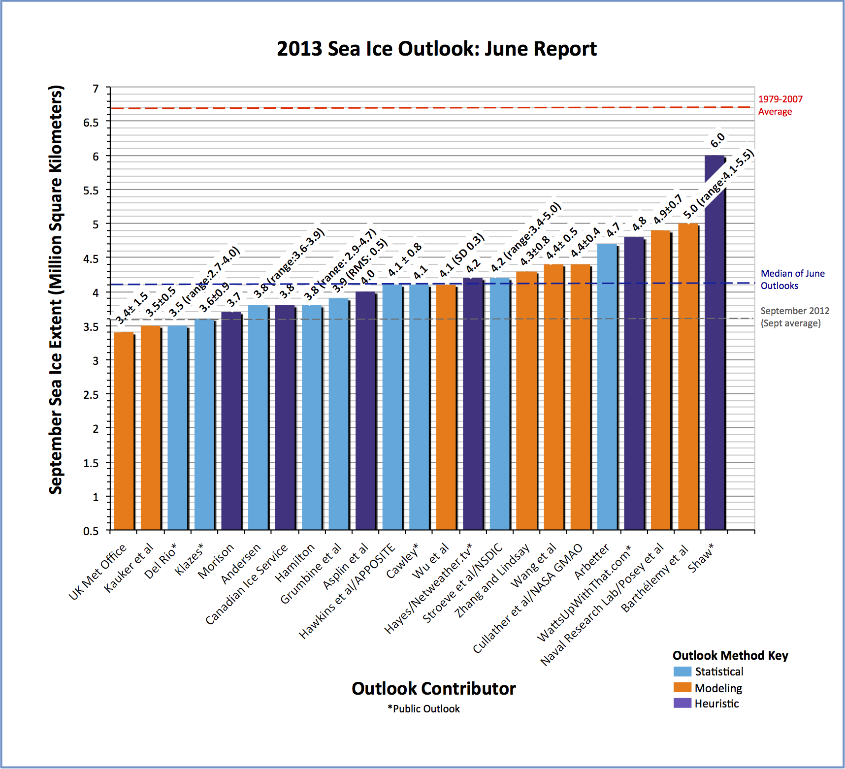
With 23 pan-arctic Outlook contributions, an increase over the last two years (thank you!), the June Sea Ice Outlook projects a September 2013 arctic sea extent (defined as the monthly average for September) median value of 4.1 million square kilometers, with quartiles of 3.8 and 4.4 million square kilometers (Figure 1).
The consensus is for an increasing downward trend of September sea ice extent. We interpret the split of 2013 Outlooks above and below the 4.1 median to different interpretations of the guiding physics: those who considered that observed sea ice extent in 2012 being well below the 4.1 level indicates a shift in arctic conditions, especially with regard to reduced sea ice thickness and increased sea ice mobility; and those with estimates above 4.1 who support a return to the longer-term downward trend line (1979-2007). It is always important to note for context that all estimates are well below the 1979–2007 September mean of 6.7 million square kilometers.
This month's report includes details on the causes of the 2012 minimum, the use of sea ice volume versus extent, sea ice in climate models, and late spring 2013 conditions. There has been a lot of discussion over the past few years on the use of sea ice volume as a better index than sea ice extent for use in Outlooks. For example, the events of summer 2012 suggest that spring sea ice extent is probably not the best variable on which to base summer Outlooks. Sea ice anomalies at the springtime maximum probably have more to do with what is happening to weather over subarctic seas rather than what is happening to preconditioning of sea ice in the Arctic Basin proper.
Individual responses continue to be based on a range of methods: statistical, numerical models, comparison with previous rates of sea ice loss, estimates based on various non-sea ice datasets and trends, and subjective information (i.e., the "heuristic" category). In addition to the 23 pan-arctic Outlooks, we have four regional Outlooks that provide more detail for the Northwest Passage, the Arctic Bridge (Hudson Bay / Hudson Strait), Nares Strait and the Lincoln Sea, and the Greenland and Barents Seas.
 for September 2013 sea ice extent (values are rounded to the tenths).")
The Pan-Arctic report was developed by Jim Overland, NOAA, and Helen Wiggins, ARCUS. The Regional report was developed by Adrienne Tivy, National Research Council Canada, with assistance from Kristina Creek, ARCUS.
Pan-Arctic Full Outlook
OVERVIEW OF RESULTS
With 23 responses, an increase over the last two years (thank you!), the June Sea Ice Outlook (based on May data) projects a September 2013 arctic sea extent median value of 4.1 million square kilometers, with quartiles of 3.8 and 4.4 million square kilometers (Figure 1). The consensus is for an increasing downward trend of September sea ice extent. This compares to observed September values of 3.6 in 2012, 4.6 in 2011, 4.9 in 2010, 5.4 in 2009, 4.7 in 2008, and 4.3 in 2007. The median Outlook for 2013 is below all previous June Outlook estimates and falls between the 2011 and 2012 observed September values. We interpret the split of 2013 Outlooks above and below the 4.1 level to different interpretations of the guiding physics: those who considered that observed sea ice extent in 2012 being well below the 4.1 level indicates a shift in arctic conditions, especially with regard to reduced sea ice thickness and increased sea ice mobility; and those who have estimates above 4.1 who support a return to the longer-term downward trend line (1979-2007). It is always important to note for context that all 2013 estimates are well below the 1979-2007 September mean of 6.7 million square kilometers.
Individual responses continue to be based on a range of methods: statistical, numerical models, comparison with previous rates of sea ice loss, estimates based on various non-sea ice datasets and trends, and subjective information (the "heuristic" category). While the summary focuses on median and quartile values from the entire set of contributions, it is important to recall that may individual estimates specify rather broad uncertainty ranges.
Outlooks are not forecasts; their purpose is to promote a discussion of the physics and factors influencing summer sea ice loss. Again in 2013, we are pleased at the range of methods and discussions and thank the increasing number of contributors for their considerable efforts. We look forward to another strong showing for the July Outlook and always welcome new contributors. The Outlook is receiving greater interest and the Outlook team plans to continue our efforts.
DISCUSSION
The Sea Ice Outlook (SIO) is well established and will continue in the future; stay tuned for further updates on planned activities. Participation and broad interest remains high. With regard to the Outlook estimates for the past three years, the median values for June outlooks for sea ice extent were within 0.1 million square kilometers (msk) of the observed values of 4.9 msk in 2010 and 4.6 msk in 2011, but the June Outlook value of 4.4 msk in 2012 was well above the extreme observed September value of 3.6 msk. However, the 2012 Outlook estimate was in the right direction, below 2008-2011 September observations (Figure 2).
The year 2007 was a "perfect storm" of atmospheric conditions for sea ice loss during all of the summer (Zhang et al. 2008, and others). While sea ice loss in 2012 had some atmospheric conditions supporting loss at the beginning of summer, the loss in 2012 probably was the result of thin sea ice initial conditions. There has been discussion of the role of an August storm in 2012; the storm contributed to breakup of the sea ice and perhaps enhanced sea ice decay. However, record loss in 2012 compared to 2007 depended more on preconditioning with thinner and more mobile sea ice field (Parkinson and Comiso 2013, Zhang et al. 2013). Thus while the sea ice community can be forgiven for not anticipating the 2007 surprise even in early summer 2007, the Outlook team as a whole could be said to have underestimated the extent of preconditioning and the potential vulnerability of the pack in 2012.
.")
Sea Ice Volume Versus Extent
Many people have commented that sea ice volume is a better index to use than sea ice extent. That is why we have included thickness and ice age information in previous years' SIO. One major paper that came out this previous winter was by Laxon et al. (2013). Using new data from CryoSat-2 validated with in situ data, they generate estimates of ice volume for the winters of 2010/11 and 2011/12 and compare these data with current estimates from the University of Washington team of sea ice hindcasts (PIOMAS) and earlier (2003–8) estimates from the ICESat mission. There is now an estimate that arctic sea ice volume has decreased by 75-80 % since the 1980s. (Figure 3). http://psc.apl.washington.edu/wordpress/research/projects/arctic-sea-ic…
What happened in summer 2012, and Figure 3, suggest that spring sea ice extent is probably not the best variable on which to base summer Outlooks. Sea ice anomalies at the springtime maximum probably have more to do with what is happening to weather over subarctic seas rather than what is happening to preconditioning of sea ice in the Arctic Basin proper. What might be more relevant is the state of basin sea ice, such as the multiple caving in the Beaufort Sea during late winter 2013 (Figure 4).
.")
.")
Sea Ice in Climate Models
Although the SIO focuses on summer seasonal Outlooks, recent information on decadal scales is relevant to near-term changes. The climate model output (CMIP5) that will contribute to the 5th Assessment Report of the International Panel on Climate Change (AR5 IPCC) are available and have been evaluated in several journal articles. The AR5 will be available in late fall 2013. Our Figure 5 from Stroeve et al. (2012) shows that 80% of the individual climate model runs have trends that are less than observations (black band). Further, most model runs reach minimum 1.0 msk summer sea ice extents in the second half of the 21st century with a median near the year 2060. The divergence in timing of sea ice loss between models and data—decades as represented by ice volume in Figure 3—is physically irreconcilable. This leaves the arctic community without a quantitative method for determining the timing of future conditions. Do we consider that arctic change has urgency over the next decade or will there not be large changes until the second half of the century? Most arctic scientists are aware of the interaction of multiple feedbacks that are not fully resolved by climate models, and thus support the need for major improvements before models can be used for quantitative estimates for the timing of future changes.
. After Stroeve et al. (2012).")
LATE SPRING 2013 CONDITIONS
We are very pleased to have an early look at sea ice thickness data from recent NASA-sponsored "IceBridge" flights. A sea ice thickness product by Nathan Kurtz, Michael Studinger, and Sinead Farrell is shown in Figure 6. While there are high values near the Greenland coast, offshore the values are variable along the aircraft flight tracts. Sea ice was generally thin (
We also have an "on the ice" report from north of Barrow by Oliver Dyre Dammann and Hajo Eicken, University of Alaska. Shorefast ice conditions along the northeastern Chukchi Sea coast (Barrow to Wainwright) reflect the combination of late freeze-up after the 2012 record minimum summer ice extent and persistent westerly flow advecting warm air throughout fall and early winter. The lack of major storms from the western/northern sector resulted in a shorefast ice cover that is potentially unstable due to the lack of grounded pressure ridges. The complete absence of multiyear sea ice in the region, confirmed by thickness surveys and local observations, is a first for the region in the past several decades. In early March, shorefast ice broke out close to the beach along a >100km stretch of coast between Barrow and Wainwright. These conditions have left shorefast ice vulnerable to break-out events. Hunters in the region have had to traverse thin, unstable ice as reflected in ice thickness surveys along trails in the Barrow region. With lack of multiyear ice, a normal or slightly below-normal thickness offshore ice cover (based on ice thickness flights earlier in the season) and coastal ice vulnerable to early break-up, ice conditions would favor a normal or somewhat early seasonal ice retreat.
Figure 7 shows a loss of sea ice extent through May 2013 (National Snow and Ice Data Center). Sea ice extent was below average in the Barents Sea on the Atlantic side of the Arctic. Greater than average ice extent prevailed on the Pacific side of the Arctic. Unlike the sea level pressure field from the last six years with the Arctic Dipole (AD), which has low pressure on the Siberian side of the Arctic and higher pressure on the North American side, May 2013 had a low pressure over the central Arctic. Since the winds generally follow the pressure contours, this pattern advected warmer air into the Barents and Kara Sea while keeping cool temperatures in Alaska (Figure 8).
.")

Sea ice was more extensive at the end of May 2012 than in the previous two years and nominally was thus not a good predictor. September Outlooks for 2013 have a larger focus on thicknesses than in previous years and half of the Outlook contributions are projecting lower values than last year. Stay tuned for next month's Outlook in July.
KEY STATEMENTS FROM INDIVIDUAL OUTLOOKS
Key statements from the individual Outlook contributions are below, summarized here by first author, Outlook value (in million square kilometers, rounded to tenths), error estimate (if provided), method, and abstracted statement. The statements are ordered from lowest to highest outlook values. Each complete individual contribution is available in the "Pan-Arctic Individual PDFs" section at the bottom of this webpage.
UK Met Office (Ann Keen et al.), 3.4 ± 1.5, Modeling (forecasting system)
The GloSea4 system has a real-time forecasting component, and an accompanying set of hindcasts which are used for bias correction and skill assessment. The hindcasts and forecasts are typically run for 7 months, using the same methodology and differing only in their initial conditions.
Kauker et al., 3.5 ± 0.5, Modeling
For the present outlook the coupled ice-ocean model NAOSIM has been forced with atmospheric surface data from January 1948 to May 31 2013. This atmospheric forcing has been taken from the NCEP/NCAR reanalysis. The ensemble model experiments all start from the same initial conditions on May 31, 2013. The model system is unchanged since the last year's outlook. Compared to the NSIDC ice extent the simulated extent is underestimated in the mean by about 0.18 million km2. This bias is added to the ensemble prediction. Likely reasons for the bias are imperfections in sea ice-ocean model and the atmospheric forcing.
Del Rio Olivier (Public), 3.5 (90% range is 2.7-4.0), Statistical
Extent is defined as a ratio between volume and thickness. Thickness and volume are modelled independently, and extent is then modelled based on this two sub models.
Klazes (Public), 3.6 (95% confidence interval of +/- 0.9), Statistical
September extent is predicted using an estimated minimum value of the PIOMAS arctic sea ice volume and a simple model for volume-extent relationship.
Morison, 3.7, Heuristic
On balance I think the ice declines will be similar to last year. Present ice thickness, extent, and ocean heat observations suggest a new record might be possible. However, the negative feedback of reduced snow cover will help extent rebound a little from the 2012 minimum
Andersen, 3.8, Statistical
My method is unchanged (and described previously) as it is based on a statistical ratio of the (minimum area)/(maximum area) for the period from 2007-2012. The numbers were very consistent for the period 2007-2011, but the relative reduction increased in 2012. To encounter for this uncertainty I now give a slight range.
Canadian Ice Service, 3.8, Heuristic
Arctic Ocean September sea ice extents (while expected to be well below the 1979‐2013 average of 6.4 million square kilometres, and while expected to continue to be near or below 4.0 million square kilometres) are therefore expected to experience a slight recovery, preventing a repeat of last year's record. Forecast was derived by considering a combination of methods.
Hamilton, 3.8 (95% confidence interval: 2.9 to 4.7), Statistical
September mean extent from a Gompertz curve representing the trend over previous years. Estimation data are the NSIDC monthly mean extent reports from September 1979 through September 2012. Thus, the September 2013 extent prediction was calculated in October 2012, almost one year in advance.
Gumbine et al., 3.9 (rms error of 0.5), Statistical
Using the same methods as in prior years -- a logistic curve growth of open water -- and the ensemble of parameters which give fits to observation with rms error less than 0.5 million km2, but now with 34 years of data, the ensemble average and rms estimates are 3.90 million km2, with rms error of 0.5 million km2.
Aspin et al., 4.0, Heuristic
Sea ice extent is greater on 05 June 2013 than a year ago, however ice thicknesses and volumes are, on average, the lowest on record. While the ice is preconditioned for another record melt the atmospheric and ice conditions observed during May 2013 have not been ideal for rapid melting, evidenced by typical rates of ice decay (NSIDC, 2013). Provided that ocean and atmospheric conditions favor rapid melting in June and July, which we feel are still likely, it is therefore hypothesized that the 2013 fall sea ice extent will achieve values comparable to those of 2012, with regional losses governed by local wind and ice conditions and dynamics.
Hawkins et al. (APPOSITE Project), 4.1 ± 0.8 (5-95% range), Statistical
Used three simple statistical approaches based on September extent data. The simplest statistical forecast for extent: 4.07± 0.75million km2 (5-95% range). Spatial forecast version: 4.04± 0.75 million km2 (5-95% range). Dynamic climatology: 3.31± 1.04 million km2 (5-95% range).
Cawley (Public), 4.1, Statistical
The projection is purely statistical, using a Bayesian technique known as Gaussian process regression (similar to Krigging). A nice feature of this model is that the credible interval on the projection widens as the projection extrapolates away from the data. Note that the sea ice extent is likely to be higher than the record September minimum in 2012 simply due to "regression to the mean", but it would not imply that there had been any "recovery".
Wu et al., 4.1 (standard deviation of 0.3), Modeling
We ran the CFSv2 model with 31 May 2013 revised-initial conditions. The initial conditions were modified from real time CFSv2 initial conditions by thinning the ice pack, similar to what we did in making our 2011 and 2012 sea ice outlook (SIO) estimate. If this thinning would have eliminated ice from areas observed to have sea ice, a minimum thickness of 20 cm was left in place for the ice initial condition.
Netweather.tv (Public), 4.2, Heuristic
Poll of Netweather.tv forum members.
NSIDC (Stroeve et al), 4.2 (range 3.4 to 5.0), Statistical
We use the survival of ice of different ages to statistically predict the 2013 minimum. Ice age fields are based on the ice age algorithm of Fowler et al. [2003]. The ice age product is based on a 15% sea ice concentration threshold to be consistent with the threshold used for mapping overall sea ice extent. In addition, the use of a 15% threshold captures greater detail within the marginal ice zone. Using this approach and taking into consideration that the survivability of ice during the summer melt season has changed in recent years, gives an estimate of 4.67 106 km2, using ice survival rates from the last 5 summers, which increases to 5.04 106 km2 using the last 10 years of survival rates. To be conservative, we use the last 10 years and give an expected range of 3.36 106 km2 (based on 2012 survival rates) to 5.04 106 km2, with an average of 4.20 106 km2. If ice survival rates are similar to those in 2012, a new record low would be reached.
Zhang and Lindsay, 4.3 ± 0.8, Model
The forecasting system is based on a synthesis of a model, the NCEP/NCAR reanalysis data, and satellite observations of ice concentration and sea surface temperature. The model is the Pan-Arctic Ice-Ocean Modeling and Assimilation System (PIOMAS). The ensemble consists of seven members each of which uses a unique set of NCEP/NCAR atmospheric forcing fields from recent years, representing recent climate, such that ensemble member 1 uses 2006 NCEP/NCAR forcing, member 2 uses 2007 forcing …, and member 7 uses 2012 forcing. In addition, sea ice thickness data from three different projects were used to correct the PIOMAS sea ice thickness distribution estimates for 1 April 2013. The data were collected between 21 March and 24 April. These projects were the NASA mission Operation IceBridge.
Wang et al., 4.4±0.5, Modeling
The CFSv2 has shown long-term decrease of sea ice extent during the past 3 decades, as in the observation. The CFSv2 was also found to have some skill in predicting year to year variability at seasonal time scales. The skill estimated as the forecast correlation with observation based on retrospective forecasts for 1982-2012 is 0.78. Forecast uncertainty taken as the RMS error based on 1982-2012 retrospective forecasts is 0.5×10⁶ km2.
Cullather et al. (NASA GMAO), 4.4 ± 0.4, Modeling
Seasonal coupled forecasts are conducted by the Global Modeling and Assimilation Office (NASA GMAO) on an experimental basis in near real time with the GEOS-5 AOGCM. Seasonal forecasts are initialized with GEOS-iODAS, MERRA-Land, and MERRA atmospheric fields. Forecasts are initialized every 5 days, with 10 ensemble members initialized on the date closest to the beginning of the month. The ensemble members are generated by coupled model breeding and by independent perturbations in the ocean and atmosphere. Sea ice extent is defined by the area in which ice concentration exceeds 15 percent.
Arbetter, 4.7, Statistical
A statistical model using regional observations of sea ice area and global NCEP air temperature, sea level pressure, and freezing degree day estimates continues the trend of projecting below-average summer sea ice conditions for the Arctic.
WattsUpWithThat.com (Public), 4.8 million km2, Heuristic
Reader poll by WattsUpWithThat.com.
Naval Research Laboratory (Posey et al), 4.9 -+ 0.7, Model
The Arctic Cap Nowcast Forecast System (ACNFS) was run in forward model mode, without assimilation, initialized with a May 1, 2013 analysis, for ten simulations using archived Navy atmospheric forcing fields from 2003-2012. The mean ice extent in September, averaged across all ensemble members, corrected for forward model bias.
Barthélemy et al., 5.0 (range from 4.1 to 5.5), Modeling
Our estimate is based on results from ensemble runs with the global ocean-sea ice coupled model NEMO-LIM3. This model has been proven skillful in reproducing the monthly arctic (and Antarctic) sea ice extent anomalies over the last 30 years, as well as the observed long-term downward trend. The ensemble members are expected to sample the atmospheric variability that may prevail this summer.
Shaw (Public), 6.0, Heuristic
I expected a swift early ice-melt, due to warmth over Greenland and Northeast Canada caused by the spring's blocking pattern, but expect a slow-down of ice melt that will be surprising to many.
CITATIONS
Laxon, S. W., and coauthors (2013), CryoSat-2 estimates of arctic sea ice thickness and volume, Geophys. Res. Lett., doi:10.1002/grl.50193.
Overland, J.E., and M. Wang (2013),When will the summer arctic be nearly sea ice free? Geophys. Res. Lett., doi: 10.1002/grl.50316.
Parkinson, C. L., and J. C. Comiso (2013), On the 2012 record low arctic sea ice cover: Combined impact of preconditioning and an August storm, Geophys. Res. Lett., 40, 1356–1361, doi:10.1002/grl.50349.
Stroeve, J., V. Kattsov, A. Barrett, M. Serreze, T. Pavlova, M. Holland, and W. N. Meier (2012), Trends in arctic sea ice extent from CMIP5, CMIP3 and observations, Geophys. Res. Lett. doi:10.1029/2012GL052676.
Zhang, J., R. Lindsay, M. Steele, and A. Schweiger (2008), What drove the dramatic retreat of arctic sea ice during summer 2007?, Geophys. Res. Lett., 35, L11505, doi:10.1029/2008GL034005.
Zhang, J., R. Lindsay, A. Schweiger, and M. Steele (2013), The impact of an intense summer cyclone on 2012 arctic sea ice retreat, Geophys. Res. Lett., 40, doi:10.1002/grl.50190.
The Pan-Arctic report was developed by Jim Overland, NOAA, and Helen Wiggins, ARCUS. The Regional report was developed by Adrienne Tivy, National Research Council Canada, with assistance from Kristina Creek, ARCUS.
| Attachment | Size |
|---|---|
| Andersen60.91 KB | 60.91 KB |
| Arbetter417.2 KB | 417.2 KB |
| Asplin et al.1.42 MB | 1.42 MB |
| Barthelemy et al.865.08 KB | 865.08 KB |
| Canadian Ice Service324.77 KB | 324.77 KB |
| Cawley26.04 KB | 26.04 KB |
| Cullather et al. (NASA GMAO)333.61 KB | 333.61 KB |
| Del Rio217.14 KB | 217.14 KB |
| Grumbine et al.43.88 KB | 43.88 KB |
| Hamilton247.14 KB | 247.14 KB |
| Hawkins et al. (APPOSITE)434.61 KB | 434.61 KB |
| Hayes (Netweather TV)66.63 KB | 66.63 KB |
| Kauker et al.875.03 KB | 875.03 KB |
| Keen et al. (UK Met. Office)636.98 KB | 636.98 KB |
| Klazes228.06 KB | 228.06 KB |
| Morison27.58 KB | 27.58 KB |
| Posey et al. (Naval Research Laboratory)700.02 KB | 700.02 KB |
| Shaw50.28 KB | 50.28 KB |
| Stroeve et al. (NSIDC)467.45 KB | 467.45 KB |
| Wang et al.65.9 KB | 65.9 KB |
| WattsUpWithThat.com51.66 KB | 51.66 KB |
| Wu et al.38.04 KB | 38.04 KB |
| Zhang and Lindsay332.28 KB | 332.28 KB |
| Attachment | Size |
|---|---|
| Gerland et al.288.48 KB | 288.48 KB |
| Gudmandsen32.04 KB | 32.04 KB |
| Tivy184.67 KB | 184.67 KB |
| Zhang and Lindsay332.28 KB | 332.28 KB |
 for September 2013 sea ice extent (values are rounded to the tenths for the graph).")