
Summary
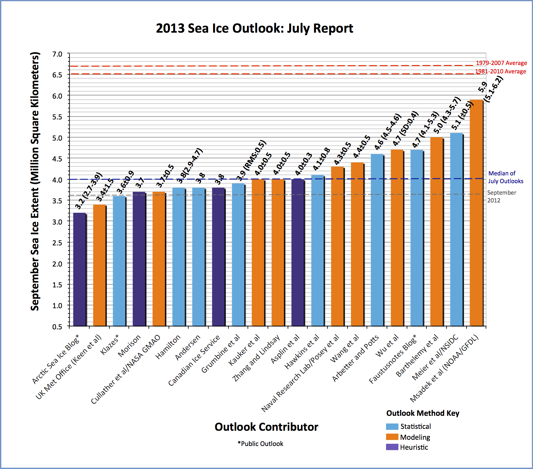
We appreciate the continuing contributions to the July Outlook (using June data). We received 21 Pan-Arctic responses for the September 2013 Arctic mean sea ice extent with a median value of 4.0 million square kilometers and the quartile values are 3.8 and 4.6 million square kilometers (Figure 1). The range of estimates was 3.2 to 5.9 million square kilometers. For comparison, the June 2013 median was 4.1 million square kilometers and the July median from 2012 was 4.6 million square kilometers. Thus the data from 2012 and recent estimates of thinning sea ice appear to have an impact in lowering Outlook estimates.
 for September 2013 mean sea ice extent (values are rounded to the tenths).")
Download High Resolution Version of Figure 1.
Individual responses continue to be based on a range of methods: statistical, numerical models, comparison with previous rates of sea ice loss, estimates based on various non-sea ice datasets and trends, and subjective information (i.e., the "heuristic" category). See Figure 2 for a comparison of different methods between June and July.
 of each group. The overall July median, 4.0 million km2, is marked by a horizontal line. The modeling and statistical predictions appear fairly stable from June to July, with the statistical predictions generally more pessimistic. Heuristic predictions shifted more substantially, reflecting a changing pool of contributors. (Courtesy of Larry Hamilton, U. of New Hampshire)")
As in 2012, sea ice thinning and not just anomalous weather should contribute to September 2013 sea ice loss.
In addition to the 21 pan-arctic Outlooks, we have 5 regional Outlooks that provide more detail for the Northwest Passage, Arctic Bridge (Hudson Bay / Hudson Strait), Laptev-Kara-Barents-Greenland Seas, Canadian Arctic Archipelago and Nares Strait.
The Pan-Arctic report was developed by Jim Overland, NOAA, Hajo Eicken, UAF, and Helen Wiggins, ARCUS. The Regional report was developed by Adrienne Tivy, National Research Council Canada, with assistance from Kristina Creek, ARCUS.
Pan-Arctic Full Outlook
OVERVIEW OF RESULTS
We appreciate the continuing contributions to the July Outlook (using June data). We received 21 Pan-Arctic responses for the September 2013 Arctic mean sea ice extent with a median value of 4.0 million square kilometers and the quartile values are 3.8 and 4.6 million square kilometers (Figure 1). The range of estimates was 3.2 to 5.9 million square kilometers. For comparison, the June 2013 median was 4.1 million square kilometers and the July median from 2012 was 4.6 million square kilometers. Thus the data from 2012 and recent estimates of thinning sea ice appear to have an impact in lowering Outlook estimates. It should be recalled that we are comparing these Outlook values to the September average sea ice extent as provided by the National Snow and Ice Data Center (NSIDC).
Download High Resolution Version of Figure 1.
Individual responses continue to be based on a range of methods: statistical, numerical models, comparison with previous rates of sea ice loss, estimates based on various non-sea ice datasets and trends, and subjective information (i.e., the "heuristic" category). See Figure 2 for a comparison of different methods between June and July.
JUNE 2012 ICE AND ATMOSPHERIC CONDITIONS
Loss rate for May and June 2013 sea ice extent was slower than May and June 2010 and 2011 and slower than June in 2012 (Figure 3). However, in late June and early July the 2013 loss rate has increased. This contrasted with 2012, which moderated in the second half of June. It should be noted that for comparisons with climatology (Fig. 4 and 5), the reference time frame (i.e., “normal”) now extends from 1981 through 2010 and hence includes recent years of substantial summer ice loss (see this NSDIC webpage with an explanation of the change).
.")
The rapid sea ice loss in early June 2012 and in other recent years was associated with the presence of the Arctic Dipole (AD) pressure pattern with high pressure on the North American side and low pressure on the Siberian side. This AD pattern quickly shifted in the second half of June 2012, however, and was replaced by a more typical low sea level pressure center over the Arctic Ocean. In 2013 the low pressure system that was over the central Arctic in May (see June 2013 Outlook discussion) continued into the first half of June. In the latter half of June and into July 2013 the low shifted more to the Atlantic sector with a hint of the AD pattern in the Canadian Beaufort Sea (Figure 4).
 for late June early July 2013 showing a weak Arctic Dipole (AD) pattern over the central Arctic Ocean, but with strong low pressure system over the Atlantic Arctic. Data are from the NCEP–NCAR Reanalysis through the NOAA/Earth Systems Research Laboratory, generated online at http://www.esrl.noaa.gov/psd/cgi-bin/data/composites/printpage.pl")
Sea ice extent for early July 2013 (Figure 5) shows anomalous open water areas in Baffin Bay, Hudson Bay, Kara Sea, and north of the Barents Sea, with substantial open water areas within the sea ice pack north of Siberia. Rather than the AD pattern being relevant and impacting the Beaufort Sea, a key factor for sea ice loss in the last month is the strong continuing positive North Atlantic Oscillation pattern bringing warm temperatures to the North of Eurasia (Figure 4).
For the September Outlook one can note the early loss of sea ice north of Eurasia, but normal meteorological conditions over the central Arctic Ocean. As in 2012, sea ice thinning and not just anomalous weather should contribute to September 2013 sea ice loss (see the discussion of the IceBridge sea ice thickness data from the June Report).
.")
KEY STATEMENTS FROM INDIVIDUAL OUTLOOKS
Key statements from the individual Outlook contributions are below, summarized here by first author, Outlook value (in million square kilometers, rounded to tenths), error estimate (if provided and rounded to tenths), method, and abstracted statement. The statements are ordered from lowest to highest outlook values. Each complete individual contribution is available in the "Pan-Arctic Individual PDFs" section at the bottom of this webpage.
Arctic Sea Ice Blog (Public: http://neven1.typepad.com/), submitted by Hamilton and Cutler, 3.2 million square kilometers, quartile 2.7 to 3.9, Heuristic
By July 5 there had been more than 200 reader comments in response to this post. Among these comments we counted 82 individual predictions, posted along with diverse rationales, evidence and lively discussion. The format placed no restrictions on numerical values, and all comments are public for anyone to study. The median value of these 82 predictions was 3.2 million square kilometers, with an interquartile range (approximately the middle 50% of predictions) from 2.7 to 3.9 million square kilometers.
UK Met Office (Keen et al), No change from June Outlook: 3.4 ± 1.5 million square kilometers, Model
Klazes (Public), 3.6 million square kilometers; 95% range +/- 0.9, Statistical
The method is based on mean September ice extent and minimum September ice volume. The ice volume data used here is the Pan-Arctic Ice Ocean Modeling and Assimilation System (PIOMAS) calculated by the Polar Science Center at the Applied Physics Laboratory of the University of Washington. Both volume and extent have been declining in the last decade, but volume has the highest signal to noise ratio. This makes it somewhat easier to predict volume than extent. If the relation between extent and volume is known, the extent may be predicted with better accuracy than a statistical model based on extent alone.
Morison, No change from June Outlook: 3.7 million square kilometers, Heuristic
Cullather et al. (NASA GMAO), 3.7 ± 0.5 million square kilometers, Model.
The projection is comparable to the September 2012 record minimum, and is less than the previous month’s contribution to the Sea Ice Outlook (4.42 million square kilometers). While the ensemble forecast indicates an absence of significant atmospheric circulation anomalies over the western Arctic, high pressure features over the Barents sea appear to be conducive to greater ice extent reductions along the Eurasian side. Observed ice extent rapidly decreased over the last week of June, and the ensemble forecast has bifurcated in response to evolving conditions with three ensemble members indicating record ice loss. For these members, greater ice cover loss is found throughout the Arctic as compared to the ensemble mean.
Hamilton, No change from June Outlook: 3.8 million square kilometers, 95% range 2.9 to 4.7, Statistical
Andersen, No change from June Outlook: 3.8 million square kilometers, Statistical.
Canadian Ice Service: No change from June Outlook: 3.8 million square kilometers, Heuristic.
Grumbine et al., No change from June Outlook: 3.9 million square kilometers, RMS of 0.5, Statistical.
Kauker et al. (AWI), 4.0 ± 0.5 million square kilometers, Model.
Compared to the June outlook the estimate has increased by about 0.47 million square kilometers.
Zhang and Lindsay, 4.0 ± 0.5 million square kilometers, Model.
These seven ensembles of the reanalysis atmospheric forcing fields, which incorporate a range of observations, may capture the climate variability expected in 2013. Each ensemble prediction starts with the same initial ice–ocean conditions on 7/1/2013. To obtain the “best possible” initial ice-ocean conditions for the forecasts, we conducted a retrospective simulation using PIOMAS that assimilates satellite ice concentration and sea surface temperature data.
Asplin et al. (CEOS), 4.0 ± 0.3 million square kilometers, Heuristic.
The mean ice concentration anomaly for June 2013 is 0.9 x 10⁶ square kilometers greater than June 2012, however Arctic sea ice thicknesses and volumes continue to remain the lowest on record. Anomalous cyclonic atmospheric circulation throughout the Arctic Basin during June has continued to precondition sea ice, making the ice cover vulnerable to a precipitous drop in sea ice extent; however the persistence of the June cyclonic circulation (and cloudiness associated with the surface lows) has induced divergence within the sea ice cover, and has delayed the onset of the rapid sea ice extent decline typically observed in June. Given the preconditioned ice cover, and short-term forecast for increased high pressure in the Arctic, it is still likely that the 2013 fall sea ice extent will achieve values comparable to those of 2007. We see July as a critical month where favorable atmospheric and oceanic conditions could rapidly erode the preconditioned Arctic sea ice cover.
Hawkins et al. (APPOSITE/U. Reading), No change from June Outlook, 4.1 ± 0.8 million square kilometers, Statistical.
Posey et al (Naval Research Lab): 4.3 million square kilometers ± 0.5, Model.
The Arctic Cap Nowcast Forecast System (ACNFS) was run in forward model mode, without assimilation, initialized with a June 1, 2013 analysis, for eight simulations using archived Navy atmospheric forcing fields from 2005-2012. The mean ice extent in September, averaged across all ensemble members, corrected for forward model bias is our projected ice extent.
Wang et al., No change from June Outlook: 4.4 ± 0.5 million square kilometers, Model.
Arbetter and Potts (NIC), 4.6 million square kilometers, range 4.5 to 4.6, Statistical.
Multiple Linear Regression statistical model.
(Ed. note: Method category corrected on 7/12).
Wu et al., 4.7 million square kilometers, standard deviation of 0.4, Model.
Our projected Arctic sea ice extent from the NCEP CFSv2 model with June 2013 revised-initial condition using 30-member ensemble forecast is (surprisingly increased to) 4.7 million square kilometers with a standard deviation of 0.4 million square kilometers.
Faustusnotes blog (Public): 4.7 million square kilometers, 95% interval 4.1 to 5.3, Statistical.
Estimated the extent value using a linear regression model and key measures of temperature, snow cover, area and extent for the current and previous years. This model has some ability to predict the previous two crashes, and suggests a large recovery of the sea ice extent this September.
Barthelemy et al. (UCL/Belgium), 5.0 million square kilometers, range 4.3 to 5.7, Model.
Our estimate is based on results from ensemble runs with the global ocean-sea ice coupled model NEMO-LIM3. Each member is initialized from a reference run on June 23, 2013, then forced with the NCEP/NCAR atmospheric reanalysis from one year between 2003 to 2012. Our estimate is the ensemble median, and the given range corresponds to the lowest and highest extents in the ensemble.
Meier et al./NSIDC, 5.1 ± 0.5 million square kilometers, Statistical.
The rationale for this method is that by the end of June, the sun is beginning to set and solar insolation is decreasing. Thus, the potential range of the ice extent evolution begins to become constrained and range of extents will encompass the likely actual trajectory this year. Comparison with previous years’ rates and climatological averages of year ranges are assessed to yield a most likely range.
Msadek et al. (NOAA/GFDL), 5.9 million square kilometers, range 5.1 to 6.2, Model.
Our estimate is based on the GFDL CM2.1 ensemble forecast system in which both the ocean and atmosphere are initialized on July 1 using coupled data assimilation. Our projection is the bias-corrected ensemble mean, and the given range corresponds to the lowest and highest extents in the 10-member ensemble. While the projected 2013 extent remains below the 1979-2007 observed average, the model predicts that September Arctic sea-ice extent will recover to a value comparable to that reached in 2006.
The Pan-Arctic report was developed by Jim Overland, NOAA, Hajo Eicken, UAF, and Helen Wiggins, ARCUS. The Regional report was developed by Adrienne Tivy, National Research Council Canada, with assistance from Kristina Creek, ARCUS.
| Attachment | Size |
|---|---|
| Andersen60.91 KB | 60.91 KB |
| Arbetter and Potts272.54 KB | 272.54 KB |
| Arctic Sea Ice Blog (Submitted by Hamilton and Cutler)145.06 KB | 145.06 KB |
| Asplin et al.3.52 MB | 3.52 MB |
| Barthelemy et al.848.69 KB | 848.69 KB |
| Canadian Ice Service75.9 KB | 75.9 KB |
| Cullather et al.334.78 KB | 334.78 KB |
| Faustusnotes Blog35.94 KB | 35.94 KB |
| Grumbine et al.43.88 KB | 43.88 KB |
| Hamilton224.37 KB | 224.37 KB |
| Hawkins et al.434.61 KB | 434.61 KB |
| Kauker et al.159.46 KB | 159.46 KB |
| Keen et al.636.98 KB | 636.98 KB |
| Klazes240.69 KB | 240.69 KB |
| Meier et al.544.77 KB | 544.77 KB |
| Morison27.58 KB | 27.58 KB |
| Msadek et al.172.81 KB | 172.81 KB |
| Posey et al.551.56 KB | 551.56 KB |
| Wang et al.65.9 KB | 65.9 KB |
| Wu et al.38.93 KB | 38.93 KB |
| Zhang and Lindsay500.34 KB | 500.34 KB |
| Attachment | Size |
|---|---|
| Gerland et al.435.04 KB | 435.04 KB |
| Gudmandsen28.95 KB | 28.95 KB |
| Kaleschke and Rickert1.73 MB | 1.73 MB |
| Tivy186.06 KB | 186.06 KB |
| Zhang and Lindsay500.34 KB | 500.34 KB |
 for September 2013 mean sea ice extent (values are rounded to the tenths).")