
Outlook Report
Executive Summary
We express our thanks to all the groups and individuals who submitted their contribution to the 2020 June Sea Ice Outlook (SIO) report during these difficult times.
We received 33 contributions of September sea-ice extent that included pan-Arctic predictions; of those contributions, eight also included predictions for pan-Antarctic and the Alaska Region (Bering, Chukchi, and Beaufort seas). Additionally, we received 13 submissions of sea-ice probability (SIP), and ten submissions of first ice-free date (IFD). What is new this year is that we added ice-free conditions for the Hudson Bay region (eight submissions) and September sea-ice concentration contour in the Fram Strait region, motivated by the MOSAiC expedition (eight submissions). Also new this year, we have invited forecast contributors to submit their forecast initial conditions (sea-ice concentration and sea-ice thickness) to better understand how observations are being used in forecasts. For the June 2020 SIO, we received four submissions of initial conditions (three from dynamical models, and one from a statistical model). The submissions show that models generally agree in their sea-ice concentration initial conditions, but there is a wide spread in their sea-ice thickness initial conditions.
For the Arctic, the median June Outlook for September 2020 sea-ice extent is 4.33 million square kilometers, with quartiles of 4.06 and 4.59 million square kilometers. To place this year's Outlook in context, the historical record September low was set in 2012 at 3.57 million square kilometers, and the second lowest record was 4.27 million square kilometers set in 2007. This year's projection is close to the 2019 June Outlook, which was 4.40 million square kilometers, and close to the observed September sea-ice extent of 4.32 million square kilometers. For September 2020, only two of the outlooks project sea-ice extent below the historical low record. Thus, there is a consensus judgement against a new record low September sea-ice extent.
There is strong agreement in predicted September sea-ice extent in 2020 among the median values of 4.35, 4.26, and 4.35 million square kilometers from the dynamical, statistical, and heuristic approaches, respectively. This is different from what we have seen in the past in that the heuristic approaches had generally lower median values and the dynamical models had generally higher September sea-ice extent values compared to the overall median. For example, in the 2019 June SIO, the median values for dynamical, statistical, and heuristic approaches were 4.57, 4.40, and 4.09 million square kilometers respectively, with a difference between the dynamical and heuristic method of 0.48 million square kilometers.
For the Alaska Region, the outlook for the combined Bering, Chukchi, and Beaufort sea-ice extent thus far in the 2020 retreat season is slightly lower than the 1981–2010 median and notably lower than the 2019 sea-ice season. Among the eight contributions, five are based on dynamical models and three are based on statistical methods. The multimodal median for the June 2020 SIO forecasts is 0.50 million square kilometers. To put these outlooks in historical perspective, the September mean sea-ice extent for the Alaska seas (Bering, Chukchi, and Beaufort), averaged over 2007–2019, is 0.44 million square kilometers.
For Hudson Bay, for the first time, we provided ice-free dates (IFD) forecast. We received eight submissions from dynamical (seven) and statistical (one) models. The multimodel mean forecast of ice-free conditions at 15% sea-ice concentration threshold suggests the southern part of the Bay will not become ice-free until mid-July, with some coastal regions not losing the fast ice until the end of July/early August.
For Fram Strait, as noted, motivated by the MOSAiC expedition aboard the German icebreaker Research Vessel Polarstern, we invited contributions of the 80% September sea-ice concentration contour in the Fram Strait region. We received eight contributions; most forecasts agree in the 80% contour being close to the June 2020 location of the R/V Polarstern.
For the Antarctic, sea-ice cover reaches its maximum extent in September. This year, eight outlooks of September mean sea-ice extent were received compared to six for last year. The eight forecasts span a range of 15.7–21.3 million square kilometers, which surpasses the range in the observed satellite record.
Contributions to the 2020 SIPN/Year of Polar Prediction community forecast experiment, the Sea Ice Drift Forecast Experiment (SIDFEx), are still being received and will be discussed when available.
This June Outlook was developed by lead authors Muyin Wang, University of Washington (Executive Summary, Overview, and discussion of current conditions) and James Overland, NOAA Pacific Marine Environmental Laboratory (PMEL; Overview and discussion of current conditions); with contributions from Edward Blanchard-Wrigglesworth, University of Washington (discussion on predicted spatial fields and Fram Strait); Michael Steele, University of Washington (discussion of ocean heat); Uma Bhatt, John Walsh, and Richard Thoman, University of Alaska Fairbanks (discussion of ice conditions in the Bering and Chukchi seas); Julienne Stroeve, National Snow and Ice Data Center (NSIDC) (discussion of ice conditions in the Hudson Bay region); Cecilia Bitz, University of Washington (discussion of ice conditions in the Hudson Bay region and spatial field figures); François Massonnet, Université catholique de Louvain (discussion of Antarctic contributions); Molly Hardman, NSIDC (statistics and graphs); Betsy Turner-Bogren, Helen Wiggins, Stacey Stoudt, and Lisa Sheffield Guy, ARCUS (report coordination and editing); and the rest of the SIPN2 Project Team.
Note: The Sea Ice Outlook provides an open process for those who are interested in Arctic sea ice, to share predictions and ideas; the Outlook is not an operational forecast.
See June Call for Contributions
Overview
The 33 Arctic June Outlook contributions for September 2020 sea-ice extent projections are based on multiple approaches (Figure 1). There were three contributions using a heuristic or qualitative analysis approach (one less than 2019), 14 using statistical methods (one more than 2019), and 16 using dynamical models, i.e., based on physics equations (two more than 2019). This year's median projected value of 4.33 million square kilometers compares to the projected value of 4.40 million square kilometers for 2019, and 4.6 million square kilometers for 2018. Two projections, both by dynamic models, are for a new record low, below the mark of 3.60 million square kilometers set in 2012. Conversely, four dynamical models predicted the September sea-ice extent above 5.0 million square kilometers.
For the Arctic, the median June Outlook for September 2020 sea-ice extent projection is 4.33 million square kilometers with quartiles of 4.06 and 4.60 million square kilometers. Projections from dynamic models have the largest spread of contributed outlooks, with a median value of 4.35 million square kilometers, and quartiles of 4.20 and 4.90 million square kilometers. This spread is larger than the contributions from statistical methods, which has quartiles of 3.96 and 4.57 million square kilometers. The median values by all three methods are close: 4.35 (dynamic), 4.26 (statistic), and 4.35 (heuristic) million square kilometers (Figure 2).
Except for the highest and the two lowest contributions, all estimates are in a narrow range. Thus, there is a collective opinion that projections should be close to persistence (based on recent observations), and against rapid large decreases in summer Arctic sea-ice extent. Figure 3 shows the historical data for September sea-ice extent. Extent for recent years is near the linear trend line. Extreme minima in 2007 and 2012 appear to be singular events forced by high temperatures and an unusual pattern of winds.


.")
Predictions from Spatial Fields: Sea-ice Probability, First Ice-free Date, and Forecasts' Initial Conditions
As in recent years, we have invited outlooks for September sea-ice probability (SIP) and first ice-free date (IFD). Additionally, SIPN2 is now computing SIP and IFD from forecasts of sea-ice concentration (SIC) submitted directly by contributors, and we encourage all groups to submit full-field SIC forecasts whenever possible. We do not bias-correct any fields.
SIP is defined as the fraction of ensemble forecasts that forecast September ice concentration in excess of 15% (for example, if just four out of eight ensemble forecasts predict in excess of 15% sea ice, the SIP is 50%). IFD is the first date in the melt season at which the ice concentration at a given location first drops below a certain threshold—this year we show forecasts of IFDs for two thresholds, 15% and 80% sea-ice concentration. We show 13 forecasts of SIP (10 dynamical, 3 statistical) and 10 forecasts of IFD (9 dynamical, 1 statistical).
Sea Ice Probability (SIP)
Forecasts of SIP (see Figure 4) show generally low sea-ice probabilities along the Laptev and East Siberian seas (with high confidence of an open Northeast Passage), however, model forecast uncertainty is significant—note the difference, e.g., between low sea ice forecasts from NOAA GFDL, UW APL, RASM and IAP LASG and higher SIP forecasts from the UK MetOffice and Navy ESPC. As seen in past years, models agree better in the Svalbard/Barents/Kara regions.
 for contributions with eleven dynamic models and a statistical method (Lamont). The standard deviations (bottom middle panel) indicate where contributions diverge. Figure courtesy of Bitz and Blanchard-Wrigglesworth.")
First Ice-Free Date (IFD)
Figures 5a and 5b show the IFD metrics from forecasts and climatology using two SIC thresholds, 15% and 80%. With either threshold, there is significant model uncertainty in timing of IFD. Interestingly, the regions of high forecast uncertainty in 15% IFD and 80% IFD are not co-located, but instead move with the region in proximity to the 15% and 80% in September SIC in nature.
(Editor's Note: Figures 5a and 5b updated on 4 August 2020.)
IFD 15%: indicate where contributions diverge. Figure courtesy of Bitz and Blanchard-Wrigglesworth. Updated on 4 August 2020.")
IFD 80%: indicate where contributions diverge. Figure courtesy of Bitz and Blanchard-Wrigglesworth. Updated on 4 August 2020.")
Forecast Initial Conditions
This year, we invited forecast contributors to submit their forecast initial conditions (sea-ice concentration and sea-ice thickness) to better understand how observations are being used in forecasts. For the June 2020 SIO, we received four submissions of initial conditions, including three from dynamical models (RASM, Navy ESPC, NOAA GFDL), and one from a statistical model (Nico Sun), shown in Figure 6.
 Sea-ice concentration (SIC, in %) initial conditions from three contributors; and (bottom row) sea-ice thickness (SIT, in meters) initial conditions from four contributors. Figures courtesy of Blanchard-Wrigglesworth.")
Figure 6 shows that models generally agree in their sea-ice concentration initial conditions, but there is wider spread in their sea-ice thickness initial conditions. All three dynamical models show realistic patterns of sea-ice thickness, with the thickest ice north of Greenland and the Canadian Arctic, though there are differences across models. Interestingly, the model with thicker sea ice (Navy ESPC) forecasts higher SIPs in Figure 4 above, relative to the two models with thinner sea ice (RASM and NOAA GFDL).
Current Conditions
Sea-ice extent for May 2020 (light blue, Figure 7) was the fourth lowest in the satellite passive microwave record (Figure 7, NSIDC). It was near the range of recent years (2016–2019), but well below May 2012, the year with the record low September extent, and the 1981–2010 median. However, the winter–spring weather and sea ice leading up to June 2020 contrast with conditions during 2018 and 2019. March 2020 had considerably greater extent. The winters of 2018 and 2019 had a wavy jet stream that brought warm air into the Arctic. By contrast, winter 2020 had a strong jet stream with its main location well south of the Arctic. The Arctic Oscillation (AO) index, a measure of the strength of the polar vortex, had record positive index values for January, February, and March (2.4, 3.4, 2.6 standard deviations). The positive AO conditions help isolate the Arctic from interactions with lower latitudes. This changed by May, with strong winds from the south into the central Arctic from Siberia leading to a sea-ice extent similar to recent years.

The early June 2020 sea-ice concentration map (Figure 8, NSIDC) shows open water and low concentration ice in the Chukchi Sea, northern Baffin Bay, far northern Barents Sea, and low concentrations along the Siberian coast. The sea level pressure plot (Figure 9) for 20 May through 12 June shows a low pressure center over the northern Kara Sea and high pressure on the Canadian side of the Arctic. Winds based on these pressure patterns from the south, to the east of the low pressure center, imply high air temperatures and low sea-ice concentration over the central Arctic Ocean. Typical winds from the east along northern Alaska support low sea-ice concentration in the eastern Beaufort and northeastern Chukchi seas.


Looking at the latest available weekly field of sea-ice age (NSIDC, Figure 10), there is only first year ice on the Siberian half of the Arctic, so the ice is likely fairly thin in the area. The May thickness anomaly map from PIOMAS (Figure 11) has thinner ice on the Siberian side compared to 2011–2018 average, with thicker ice on the Atlantic and North American side. Along the Chukchi coastlines, sea ice in PIOMAS is thicker than usual, somewhat at odds with the wind field and ice extents (Figures 9 and 12).

. Figure courtesy of PIOMAS.")

The 21–27 June one-week forecast of the height of the 500 hPa surface from the Climate Forecast System (Figure 13) shows a maintenance of high geopotential heights (a warm troposphere, generally implying warm conditions at the surface) and weak winds (height contours are spaced far apart) over the central and Arctic (solid green contours of 500 hPa geopotential heights and red for positives anomalies). This high pressure feature will tend to support continued loss of sea ice in this western Arctic region through at least late June.
 over the Arctic and North America. NOAA/NWS product. The dashed color contours are the anomalies relative to its climatology. Figure courtesy of the Climate Forecast System.")
In summary, the situation thus far in the 2020 retreat season and the available projections point towards substantial summer ice loss. Sea ice extent for the Arctic as a whole is already well below average. However, the atmospheric circulation pattern can change during the summer, with a corresponding impact on the rate of sea-ice retreat. The Arctic Climate Forum-5 Consensus Statement, for comparison, completed by the World Meteorological Organization (WMO) calls for below-average sea-ice extent throughout the Arctic, except for above average extent in northern Barents and Greenland seas.
Ocean Heat
This early in the summer, most of the Arctic Ocean is still ice-covered, although with significant thinning and some nascent areas of open water on the shelves. Ocean inflow to the Arctic Ocean from the North Atlantic via the Barents Sea is close to climatology based on sea surface temperature anomalies (Figure 14), although the southern Barents and Kara seas are warm. In contrast, the Pacific Ocean inflow to the Arctic Ocean is anomalously warm in the Bering and Chukchi seas (see also Figure 15b). Examination of Figure 15b indicates separate warm anomalies in the eastern Bering and northeastern Chukchi, a fairly common situation that arises from different processes in these regions. The northeast Chukchi warming is forced by easterly springtime winds that thin and then open the ice, even while areas to the south are still ice-covered. Atmospheric heating then warms the open water. As summer progresses, this isolated warm area will merge with warm water advected into the region from the south. Finally, note the anomalously cold SSTs in the eastern Beaufort Sea in Figure 15b (also barely evident in Figure 14), which are likely the result of anomalously thick ice in this area (Figure 11) that has delayed ice opening, in spite of easterly May/June winds (Figure 9).
 anomaly for 16 June 2020, relative to an average of that day over the years 1971–2000, using NOAA's OISST product, from the University of Maine Climate Change Institute's Climate Reanalyzer.")
Regional Sea-ice Extent Discussions
Alaska Region
The combined Chukchi and Beaufort sea-ice extent thus far in the 2020 retreat season is slightly lower than the 1981–2010 average (Figure 15a) and notably slower than the 2019 sea-ice season. The 15 June sea ice extent in the Chukchi Sea was 0.68 million square kilometers, which is lower than the 1981–2010 median of 0.76 million square kilometers. The 15 June sea ice extent in the Beaufort Sea was 0.92 million square kilometers and matches the 1981–2010 median value. The rate of retreat may speed up later, since May 2020 was the warmest on record in western Alaska and current sea surface temperatures are anomalously warm (Figure 15b).
, 2020 (red), 2019 (green), and 1981–2010 median (black). Image courtesy of Richard Thoman, IARC/UAF.")

The record warmth over western Alaska in May was favored by an atmospheric circulation pattern with anomalous offshore airflow, bringing warmer continental air to Alaska's western coast and offshore waters (Figure 16). The offshore flow pattern also favored the breakup of sea ice in the northern Bering and Chukchi seas. The circulation pattern represents a striking reversal from the positive AO pattern that dominated the Arctic during winter and early spring, with associated negative sea atmospheric pressure anomalies north of Alaska. The change of the circulation pattern from April to May highlights the large-scale circulation's strong variability during the winter-to-summer transition, and seasonal predictions of the summer atmospheric circulation over the Arctic have shown little skill to date.

For further information about the Climate Reanalyzer, see here.
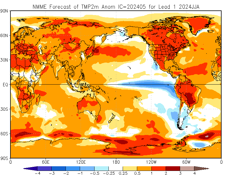
Figure 17 is a forecast map of surface air temperature anomalies for July–September 2020, based on the North American Multi-Model Ensemble (NMME), a collection of seven global forecast models run by centers in the United States and Canada. Above-average temperatures are forecast for the entire Arctic, and especially for the Chukchi Sea where the anomalies in the three-month mean exceed 2 degrees C. All but one of the seven models in the NMME predict above-average temperatures in the Alaskan seas for July–September. The International Multi-Model Ensemble (IMME) also predicts above-average temperatures in the region. It should be noted, however, that forecast air temperature anomalies over the Arctic seas are influenced at least as much by the models' ocean temperatures and presence/absence of sea ice as by the advection of temperatures by the atmospheric circulation.
 based on the NMME forecasts for July–September 2020. Source: NOAA Climate Prediction Center.")
For further information about the NOAA Climate Prediction Center see here.
For Alaskan regional sea-ice extent prediction, among the eight contributions received, three are based on statistical methods, and five are based on dynamical models (Figure 18). The dynamical model projections range from 0.14 to 1.03 million square kilometers with a mean of 0.518 million square kilometers. The statistical model projections range from 0.42 to 0.56 million square kilometers with a mean of 0.50 million square kilometers. The multimodal median for the June 2020 SIO forecasts is 0.5 million square kilometers. To put these forecasts in historical perspective, the September mean sea ice extent for the Alaska seas (Bering, Chukchi, and Beaufort) averaged over 2007–2019 is 0.44 million square kilometers (Figure 19) .

 from 1979–2019. Figure courtesy of Uma Bhatt.")
Hudson Bay
As of 21 June, Hudson Bay sea-ice extent stands at 921,706 square kilometers. This is slightly less than the 1981–2010 climatological mean value of 1.03 million square kilometers, and less than at this time of the year since 2013 (except for 2017). The least amount of sea ice in Hudson Bay for this time of year occurred in 1999. Thus far this year, the sea ice has primarily retreated within the northern part of the Bay, and also within James Bay in the south. Open water is also developing in the eastern part of the Bay. Air temperatures thus far in June have been overall below average (1 to 2 degrees Celsius) over the southern Hudson Bay and near average in the northern part. This is in stark contrast to 1999 when air temperatures were 1 to 4 degrees Celsius above average throughout most of the region.
Figure 20 shows IFD forecasts for the Hudson Bay region, which is the date when sea-ice concentration first reaches 15% (top panel, Figure 20a) and 80% (lower panel, Figure 20b). Forecasts generally show the expected retreat of ice first in the northern part of the bay, with earlier IFDs there. The multi-model mean forecast of ice-free conditions at 15% sea-ice concentration threshold suggests that the southern part of the bay will not become ice-free until mid-July, with some coastal regions not losing the fast ice until the end of July/early August. All but the UC Louvain model forecast IFD lagging the 10-year climatology, with the multi-forecast mean lagging climatology by up to about two weeks.
(Editor's Note: Figures 20a and 20b updated on 4 August 2020.)
 forecasts for a 15% sea ice concentration threshold for the Hudson Bay. The standard deviations (last panel) indicate where contributions diverge. Figure courtesy of Bitz and Blanchard-Wrigglesworth. Updated on 4 August 2020.")
 forecasts for a 80% sea ice concentration threshold for the Hudson Bay. The standard deviations (last panel) indicate where contributions diverge. Figure courtesy of Bitz and Blanchard-Wrigglesworth.")
Fram Strait
This year, motivated by the MOSAiC expedition aboard the German icebreaker, Polarstern, we invited contributions of the 80% September sea-ice concentration contour in the Fram Strait region. This value represents closed pack sea ice. Figure 21 shows forecasts from eight different models, together with the current (18 June 2020) location of the Polarstern/MOSAiC (we note that the AWI Consortium Fram Strait forecast is bias-corrected separately to the AWI Consortium SIP and IFD forecasts shown above).


Most forecasts agree that the 80% contour is close to the current location of the MOSAiC ship. Considering the climatological drift of sea ice from north to south in the Fram Strait, and the current forecasts of R/V Polarstern location, it is thus likely that by September, the location of MOSAiC will be outside the region of 80% sea-ice concentration. The multi-model mean forecasts an ice-free date (using a 80% SIC threshold) in late July–early August in this region (see IFD figure 5 above), although we note considerable forecast uncertainty.
Antarctic Contributions
This year, eight outlooks of September mean sea-ice extent were received (compared to six for last year). These span a range of 15.7–21.3 million square kilometers (Figure 22), which largely surpasses the range in the observed satellite record. This is a remarkable range compared to the Arctic submissions. From the (small) ensemble available, it can be surmised that the prediction systems taken together will probably not outperform a climatological or an anomaly persistence-based forecast. The next set of submissions (July and August) may be telling in this regard.
Caution should be exercised in interpretation of the results as the circumpolar sea-ice extent is a diagnostic with little physical relevance. The sister project of SIPN2, the Sea Ice Prediction Network South (SIPN South) aims at analyzing in more detail the (summer) Antarctic sea-ice forecasts, understanding the regional expressions of forecast biases, and preparing the ground for delivering information that is more tailored to end users.
The Sea Ice Outlook has been accepting Antarctic contributions since 2017. It is fair to say that multi-model forecast uncertainty has remained unchanged for these Antarctic outlooks.

References
Schweiger, A., R. Lindsay, J. Zhang, M. Steele, and H. Stern. 2011. Uncertainty in modeled Arctic sea ice volume. J. Geophys. Res., (doi:10.1029/2011JC007084).
Contributor Key Statements, Summary of Uncertainties
Summary Table of Key Statements from Individual Outlooks (195 KB)
Contributor Full Report PDFs and Supplemental Material
This report was developed by the SIPN2 Leadership Team
Report Leads
Muyin Wang, University of Washington and the Joint Institute for the Study of the Atmosphere at the University of Washington
Jim Overland, NOAA/Pacific Marine Environmental Laboratory
Additional Contributors:
Richard Thoman, Alaska Center for Climate Assessment and Policy, International Arctic Research Center, University of Alaska
Molly Hardman, Cooperative Institute for Research in Environmental Sciences at the University of Colorado Boulder, NSIDC
Editors:
Betsy Turner-Bogren, ARCUS
Helen Wiggins, ARCUS
Stacey Stoudt, ARCUS
Lisa Sheffield Guy, ARCUS
Suggested Citation:
Wang, M. and Overland, J.E., U.S. Bhatt, P. Bieniek, E. Blanchard-Wrigglesworth, H. Eicken, M. Hardman, L. C. Hamilton, J. Little, F. Massonnet, W. Meier, M. Serreze, M. Steele, J. Stroeve, R. Thoman, J. Walsh, and H. V. Wiggins. Editors: Turner-Bogren, B., L. Sheffield Guy, S. Stoudt, and H. V. Wiggins. June 2020. "Sea Ice Outlook: 2020 June Report." (Published online at: https://www.arcus.org/sipn/sea-ice-outlook/2020/june)
This Sea Ice Outlook Report is a product of the Sea Ice Prediction Network–Phase 2 (SIPN2), which is supported in part by the National Science Foundation under Grant No. OPP-1748308. Any opinions, findings, and conclusions or recommendations expressed in this material are those of the author(s) and do not necessarily reflect the views of the National Science Foundation.
