
Full Outlook Report
Summary
Thank you to the groups that contributed to the 2015 July Arctic Sea Ice Outlook report. We have 35 contributions (one regional only), which has beat June for a new record number of submissions.
This July Outlook report was developed by lead author Walt Meier (NASA Goddard Space Flight Center) with contributions from the rest of the SIPN leadership team, and with a section analyzing the model contributions by François Massonnet (Université catholique de Louvain and Catalan Institute of Climate Sciences).
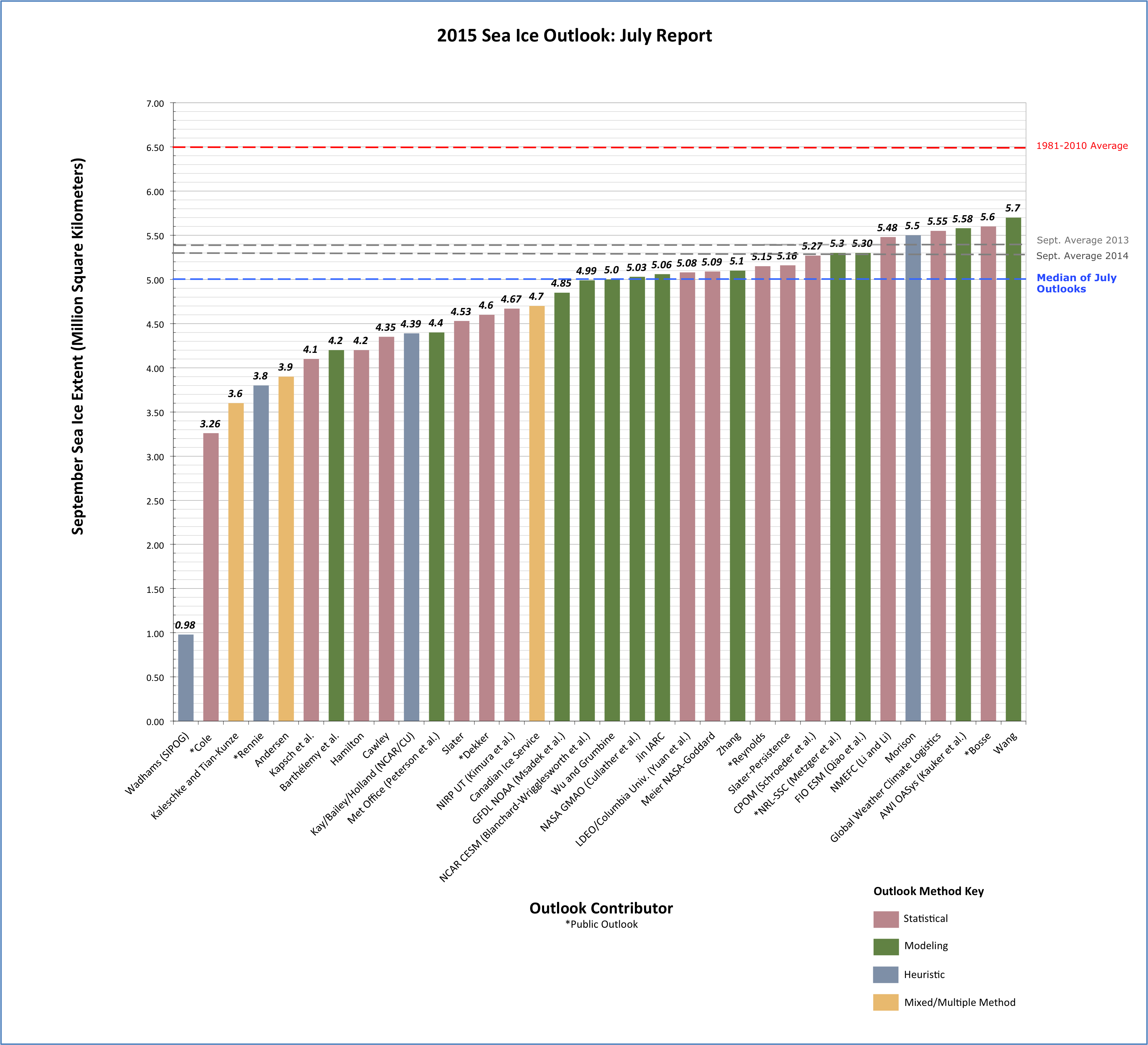
The median Outlook for September 2015 Arctic sea ice extent is 5.0 million square kilometers (km2), which is the same as the June Outlook median. The quartile range is 4.4 to 5.2 km2 (see Figure 1 in the Overview section, below). Contributions are based on a range of methods: statistical, numerical models, estimates based on trends, and subjective information. The overall range (excluding an extreme outlier) is 3.3 to 5.7 million km2. The median Outlook value is up from the July 2014 median value of 4.8 million km2. These values compare to observed values of 4.3 million km2 in 2007, 4.6 million km2 in 2011, 3.6 million km2 in 2012, and 5.3 million km2 in 2014. In general, the heuristic approaches forecast a mean September extent around 4.1 million km2, whereas the statistical and dynamical modeling approaches both suggest mean September extent near 5.1 million km2, with the dynamical modeling contributions showing a narrower range.
The lack of significant change between this month and last is largely related to the fact that most contributors did not change their forecast for July. Another factor could be the lack of significant atmospheric or oceanic forcing that would result in a large change from the June forecasts. A discussion of 11 dynamical model contributions shows no major differences compared to last month's report. This month's report also includes results from three regional predictions and a discussion of current ice and atmospheric conditions.
Overview
The Arctic Sea Ice Outlook contributions this July are based on a range of methods: statistical, numerical models, estimates based on trends, and subjective information. We again have a record number of contributions (35, one of which is regional only) and value the diversity they include. The median July Outlook for September 2015 Arctic sea ice extent is 5.0 million square kilometers (km2), which is the same as the June Outlook median. The quartile range is 4.4 to 5.2 km2 and the overall range (excluding an extreme outlier) is 3.3 to 5.7 million km2.
 for September 2015 sea ice extent.")
Download a high-resolution version of Figure 1.
In general the heuristic approaches forecast a mean September extent around 4.1 million km2, whereas the statistical and dynamical modeling approaches both suggest mean September extent near 5.1 million km2, with the dynamical modeling contributions showing a narrower range.

While many groups chose to stay with their original (June) estimate for July, 13 of the 32 June contributions did update their September extent projection (Table 1). Of these 13, some July estimates were higher while others were lower. The largest increase in forecasted September extent from the June to July Outlooks came from the heuristic forecast by Morison, which reported an increase of 700,000 km2, from 4.8 to 5.5 million km2. This increase was based on the June ice extent remaining within 1 sigma of the 1981-2010 long-term mean and nearly average melt pond coverage compared to recent years. The largest decrease from June to July Outlooks was from GFDL NOAA, which decreased by 320,000 km2, from 5.17 to 4.85 million km2. The decrease is related to a change in initial oceanic and atmospheric conditions compared to last month. Note that 6 of the 13 updated contributions show a decrease, whereas the other 7 show an increase.
| Contribution | July | June | Change |
|---|---|---|---|
| Barthélemy et al. | 4.2 | 4.5 | -0.3 |
| Dekker | 4.6 | 4.9 | -0.3 |
| NIRP UT | 4.67 | 4.58 | 0.09 |
| GFDL NOAA | 4.85 | 5.17 | -0.32 |
| Wu and Grumbine | 5 | 4.6 | 0.4 |
| LDEO/Columbia | 5.08 | 4.99 | 0.09 |
| Zhang | 5.1 | 5.2 | -0.1 |
| Slater-Persistence | 5.16 | 5.22 | -0.06 |
| CPOM | 5.27 | 5.1 | 0.17 |
| NRL-SSC | 5.3 | 5.2 | 0.1 |
| Morison | 5.5 | 4.8 | 0.7 |
| GWCL | 5.55 | 5.54 | 0.01 |
| AWI OASys | 5.58 | 5.67 | -0.09 |
There were five contributions submitted to the July report by groups who did not submit in June (Table 2). Interestingly, the median of just these five new contributions was the same as the overall median for the outlook this month — 5.0 million km2.
| Contributor | July Outlook |
|---|---|
| Cawley | 4.35 |
| Slater-Model | 4.53 |
| NCAR CESM (Blanchard-Wrigglesworth) | 4.99 |
| Meier NASA Goddard | 5.09 |
| FIO ESM (Qiao et al.) | 5.3 |
Comment on Dynamical Model Contributions
Provided by François Massonnet, Université catholique de Louvain, Belgium, & Catalan Institute of Climate Sciences, Spain
We received 12 outlooks from dynamical modeling groups; six of them have updated their predictions since the June Outlook, based on new information available in the meantime. The median of predicted September extents (all model contributions) is 5.08 million km2 (5.07 million km2 for the June Outlook). Of these, 4 predict a slight decrease (mean of 20,000 km2) compared to the June Outlook and 2 a slight increase (25,000 km2). The decrease or increase in predictions occurs from changes in the sea ice, atmospheric, and oceanic conditions used to initialize the models. For example, the change in Outlook for September extent from Barthélemy et al. is based on using June atmospheric fields to run the forecast, whereas the Zhang forecast updates sea ice concentrations and sea surface temperature (SST) fields.
Inter-model standard deviation (0.41 million km2) and estimated mean standard deviation of individual model submissions (0.49 million km2) remain comparable to the June outlook values (0.41 and 0.45 million km2, respectively), according to the same analysis as performed in the previous report.
To conclude, there is no major difference to note compared to last month's report. The statement in the last year's post-season report that models become more confident individually and as a group as time progresses has still to be confirmed. We are looking for more updated contributions for the August outlook.
 and from all other methods (grey) for the July Outlook. Values for June are shown in lighter colors. The dots are the outlook themselves and the intervals are the uncertainty ranges provided by the groups. Definitions of uncertainty were left to the discretion of the groups themselves, and should therefore be compared with caution. The middle dashed horizontal line is the median of the July outlooks from dynamical modeling groups. The lower (upper) dashed horizontal line is the lowest (largest) bound when all dynamical modeling contributions are considered. Figure courtesy of François Massonnet.")
Comment on Regional Predictions
We received two updated regional predictions and one new submission. Compared to the last ten years of climatology, the sea ice probability (SIP) values from Blanchard-Wrigglesworth et al (Figure 4) tend to be higher in the Beaufort Sea, and slightly lower in the Laptev Sea. These regional patterns are a result of regional ice thickness anomalies at forecast initialization.
 map of the projected NCAR CESM1 September mean ice extent for 2015. Image courtesy of Ed Blanchard-Wrigglesworth.")
The SIP and ice free dates from the Naval Research Laboratory (NRL) Stennis Space Center (Figure 5) have changed relatively little when compared to the June Outlook submission. The main difference is an expectation of higher SIPs in the East Siberian sea in the July outlook submission.
 map of the projected GOFS 3.1 September mean ice extent for 2015. On right: First ice-free ordinal date, with grey indicating a data void (i.e., no ice free days as the most likely outcome) of the projected GOFS 3.1 ensemble September mean for 2015. Images courtesy of NRL Stennis Space Center.")
Additionally, Gudmandsen provided an updated assessment of conditions in Nares Strait. Here, the ice barrier in the western Kane Basin has begun breaking up on the 4th of July, two weeks later than predicted in the June outlook. Despite the high temperatures observed in the area during June, it is likely that the cold winter contributed to a thicker ice cover that led to a later break up. Gudmandsen predicts that with the break-up of the ice barrier, ice transport from the Arctic through Nares strait will resume before the end of July.
Current Conditions
Overall, sea ice extent declined at a slightly slower rate than normal (relative to the 1981-2010 average rate) during June (Figure 6), losing a total of 1.6 million km2 as noted in NSIDC's Arctic Sea Ice News and Analysis report. This near normal rate of ice loss in June contributed to the upward revision in some Outlook contributions despite the extent being at record low values at the beginning of the month. However, despite near normal rates of ice loss during the month, June 2015 was a relatively warm month (Figure 7) with 925 hPa air temperatures up to 2.5 C higher than average near the North Pole and East Siberian Sea, with even warmer air temperatures in the Kara Sea (up to 4.5 C).
, 2012 (dashed green), and the 1981-2010 average (black) and standard deviation (gray). From the NSIDC Arctic Sea Ice News and Analysis.")

The air temperature patterns were a result of low pressure on the Eurasian side of the Arctic (Figure 8), along with high pressure in the Bering Sea, which supported some warm air advection into the Chukchi and East Siberian seas region. Warm conditions in the Kara Sea were consistent with low pressure centered over the Barents Sea, together with high pressure over Greenland that brought warm winds from the south. The situation changed during the first half of July with a strong dipole pattern of low pressure over the Eurasian coast and high pressure over the North Pole (Figure 9). Temperatures north of Greenland reached nearly 6C during the first two weeks of July, which has likely played a role in speeding up the ice loss during the first half of July. Currently (as of July 19), the extent is within 600,000 km2 of that in 2012 and the ice cover has become diffuse (low ice concentrations) within the Beaufort Sea (Figure 10). Ice extent remains below normal in the Kara and Barents seas, as well as in the Chukchi and East Siberian seas. In response to early retreat of sea ice within the Chukchi Sea, SSTs were fairly warm with 5+ C surface temperature anomalies, as indicated in NOAA SST analyses and UpTempO buoys (Figure 11). The waters on the Atlantic side were somewhat cooler near the ice edge with temperatures mainly 0.5-1.0 C.


 UpTempO buoys.")
Key Statements/Executive Summaries From Individual Outlooks
The Outlooks are listed below in order of lowest to highest predicted September extent. Extent and uncertainty (in parentheses) values are provided below in units of millions of km2 unless noted otherwise. The individual outlooks can be downloaded as PDFs at the bottom of this webpage.
Wadhams (Sea Ice and Polar Oceanography Group), 0.98, Heuristic (same as June)
We use entirely statistical extrapolation methods based on measured values of sea ice extent (from satellites) and sea ice thickness (from submarine voyages).
[Editor's Note: Upon review by the SIPN team, this outlook has been listed as heuristic in the Sea Ice Outlook report.]
Cole, 3.26, Statistical
Same as June contribution. Reanalysis data and satellite images agree with the snow cover forecast used to make that projection, so no change is warranted.
Kaleschke and Tian-Kunze, 3.6 (+/- 0.7), Heuristic/Statistical (same as June)
Based on February/March SMOS sea ice thickness and September SSMI sea ice concentration we provide a heuristic/statistical guesstimate for the 2015 September sea ice extent: 3.6 +/- 0.7. We use the product of the long-term average September SSMI ASI sea ice concentration and the February/March SMOS sea ice thickness as a predictor for the September extent. A threshold h applied on the (thickness Feb = Mar concentration Sept) field yields the predicted September extent after the regression with the past four years of sea ice extent observations. A threshold of h = 1.05m resulted in a correlation of R2 = 0.96 for the four years 2011, 2012, 2013 and 2014. The method applied to February/March 2015 predicts 2.8 million km2 for September. Our guesstimate is the average of the SMOS based prediction and the long term trend (4.3 million km2) with the difference of both as uncertainty.
Rennie, 3.8 (+/- 0.6), Heuristic
This estimate is primarily based on the distribution of the April PIOMAS sea ice volume estimate taking into account the extent of ice represented by various thicknesses. There appears to be a fairly consistent rate of loss measured by original thickness through until the end of July. Predicting the final figure for mid- September is much more problematic and is heavily influenced by June to Sept weather. The methodology is similar to the starting point for my estimate last year which proved to be extremely low. This years' estimate is modified to accommodate additional factors and takes into account last years' experience and factors that may have resulted in that figure being too low. These include:
a. The importance of a sequence of warm years to prepare the ice for a significant melt season.
b. The summer temperatures from May-Sept.
c. The April extent that was covered by ice estimated at between 1.5 and 2.5 m thick which, according to this methodology, would melt out at the end of the season.
d. The observation that over the past 15 years there appears to be a developing correlation between the duration when the extent is within 200 km2) of the winter maximum and the depth of the decline.
Andersen, 3.9, Statistical/Heuristic (same as June)
I continue to use the same method based on the maximum area in spring at the relatively stable reduction fraction we have seen the last 8 years. Based on the data produced by NERSC my prognosis for minimum value of the area for 2015 is 3.9 million km2. That implies just slightly more than the then record low of 2007. For more description on the method used by Andersen, please see the Andersen PDF from the 2012 SIO.
Kapsch et al., 4.1 (+/- 0.5), Statistical (same as June)
For the prediction of the September sea-ice extent we use a simple linear regression model that is only based on the atmospheric water vapor in spring (April/May). Thereby we assume that the spring atmospheric conditions, more precisely the greenhouse effect associated with the water vapor in the atmospheric column, are important for the seasonal prediction of the September sea-ice extent.
Barthélemy et al., 4.2 (3.1-4.7), Modeling
Our estimate is based on results from ensemble runs with the global ocean-sea ice coupled model NEMO-LIM3. Each member is initialized from a reference run on June 30, 2015, then forced with the NCEP/NCAR atmospheric reanalysis from one year between 2005 to 2014. Our estimate is the ensemble median, and the given range corresponds to the lowest and highest extents in the ensemble.
Hamilton, 4.2 (+/- 1.0), Statistical
A Gompertz (asymmetric S curve) model estimated by iterative least squares, looking one year ahead, suggests a mean September 2015 ice extent of 4.2 million km2. Past variations suggest a 95% confidence interval for this prediction ranging from 3.2 to 5.2 million km2 (+/- 1.0).
Cawley, 4.35 (+/- 1.16), Statistical
This is a purely statistical method (related to Krigging) to estimate the long term trend from previous observations of September Arctic sea ice extent. As this uses only September observations, the prediction is not altered by observations made during the Summer of 2015.
Kay et al. (NCAR), 4.39 (+/- 0.45), Heuristic
An informal pool of 30 climate scientists in early June 2015 estimates that the September 2015 ice extent will be 4.39 million sq. km. (std dev. 0.45, min. 3.25, max. 5.15). Since its inception 8 years ago, the NCAR/CU sea ice pool has easily rivaled much more sophisticated efforts based on statistical methods and physical models to predict the September monthly mean Arctic sea ice extent (e.g. see appendix of Stroeve et al. 2014 in GRL doi:10.1002/2014GL059388 ; Witness the Arctic article by Hamilton et al. 2014 http://www.arcus.org/witness-the-arctic/2014/2/article/21066). We think our informal pool provides a useful benchmark and reality check for Sea Ice Prediction efforts based on more sophisticated physical models and statistical techniques.
Met Office (Peterson et al.), 4.4 (+/- 0.9), Modeling (same as June)
Using the Met Office GloSea5 seasonal forecast systems we have generated a model based mean September sea ice extent outlook of (4.4 +/- 0.9) million km2. This has been generated using start-dates between 30 March and 19 April to generate an ensemble of 42 members.
Slater, 4.53 (+/- 0.52), Statistical
I have extended my forecast method to an 85-day lead time so as to forecast all days in September. The method does have a low level of real skill (taken over 1995-2013). Results contain a large uncertainty at this lead time. The current ice situation is interesting as there is a very large portion (ESS, Chukchi, and Beaufort) with mid-range concentrations and recent warmth: http://cires1.colorado.edu/~aslater/ARCTIC_TAIR. Might we see a rapid loss of ice extent in the near future? My 50-day forecast suggests so.
Dekker, 4.6 (+/- 0.37), Statistical
The basic concept behind my method pertains to estimating albedo-based Arctic amplification during the melting season. I use the "whiteness" of the Arctic in June as a predictor for how much ice will melt out between June and September. Specifically, I use a formula based on physics of energy absorption, using snow cover, and June ice extent/area numbers. The interesting result is that not only the standard deviation (at 370 k km^2) is significantly better than the 500 k km^2 or so that would be achieved for a simple linear trend, but also this method explains a large part of the increase in September ice extent during the 2013 and 2014 season w.r.t. 2012 and other years. For 2015, this method predicts that there will NOT be a repeat of the 2013 and 2014 5 million+ extent, but instead ice extent in September will be 4.6 million km^2 (+/- 370 k km^2).
NIPR/UT (Kimura et al.), 4.67, Statistical
The monthly mean ice extent in September will be about 4.67 million km2. Our estimate is based on a statistical way using data from satellite microwave sensor. We used the ice thickness in December, ice movement from December to April, and ice concentration in June. Predicted ice concentration map from July to September is available in our website: http://www.1.k.u-tokyo.ac.jp/YKWP/2015arctic2_e.html.
Canadian Ice Service, 4.7 (+/- 0.2), Heuristic/Statistical (same as June)
The 2015 forecast was derived by considering a combination of methods: 1) a qualitative heuristic method based on observed end-of-winter Arctic ice thickness extents, as well as winter Surface Air Temperature, Sea Level Pressure and vector wind anomaly patterns and trends; 2) a simple statistical method, Optimal Filtering Based Model (OFBM), that uses an optimal linear data filter to extrapolate the September sea ice extent timeseries into the future and 3) a Multiple Linear Regression (MLR) prediction system that tests ocean, atmosphere and sea ice predictors. The average forecast value of the three methods combined is 4.7 million km2.
GFDL NOAA (Msadek et al.), 4.85 (+/- 0.30), Modeling
Our prediction for the September-averaged Arctic sea ice extent is 4.85 million km2, with an uncertainty range going between 4.37 and 5.57 million km2. Our estimate is based on the GFDL CM2.1 ensemble forecast system in which both the ocean and atmosphere are initialized on July 1 using a coupled data assimilation system. Our prediction is the bias-corrected ensemble mean, and the given range corresponds to the lowest and highest extents in the 10-member ensemble. Our model predicts that September 2015 Arctic sea ice extent will be 2.11 million km2 below the 1982 to 2011 observed average extent, but will not reach values as low as those observed in 2007 or 2012.
Blanchard-Wrigglesworth et al. (NCAR CESM), 4.99 (+/- 0.47), Modeling
Our July Outlook for September 2015 is 4.99 million sq km. We have used the NCAR CESM global fully coupled model to make this prediction. Our uncertainty is 0.47 million sq km.
Wu and Grumbine, 5.0 (+/- 0.67), Modeling
The projected Arctic minimum sea ice extent from the NCEP CFSv2 model with revised CFSv2 May and June ICs using 61-member ensemble forecast is 5.04 million km2 with a SD of 0.67 million km2. The Minimum and maximum values for the Arctic sea ice extent from the 61-member ensemble prediction are 3.67 and 6.42 million km2, respectively.
NASA GMAO (Cullather et al.), 5.03 (+/- 0.41), Modeling
The GMAO seasonal forecasting system predicts a September average Arctic ice extent of 5.03±0.41 million km2, about 4.7 percent less than the 2014 value. The forecast suggests reductions in ice extent along the Eurasian coast, but cooler near-surface air temperatures over the Canadian Archipelago. A positive summertime sea level pressure anomaly over the central Arctic Basin is featured. A significant aspect of the forecast is an exuberant prediction for strengthening of the current El Niño/Southern Oscillation (ENSO) warm phase and its accompanying interaction with the Pacific-North American mode at higher latitudes. This aspect and the proximity of the ENSO spring predictability barrier to the forecast initial time implies some additional uncertainty in this year's sea ice prediction.
Jin (IARC), 5.06, Modeling (same as June)
A coupled ice-ocean model forecast of the September sea ice extent minimum.
Yuan et al. (LDEO Columbia University), 5.08 (+/- 0.51), Statistical
The prediction is made by statistical models, which are capable to predict Arctic sea ice concentrations at grid points 3-month in advance with reasonable skills. The models employ 34 years of monthly time series of sea ice, SST and atmospheric variables. The pan Arctic SIE calculated from predicted ice concentration in September 2015 is projected to be 5.08 million km2, lower than the observed extents in 2013 and 2014, but still above the historical low in 2012. The ice concentration is significantly below the 34-year climatology in the Beaufort Sea, Chukchi Sea, East Siberian Sea, Laptev Sea, Kara Sea and Barents Sea.
Meier (NASA Goddard), 5.09 (+/- 0.62), Statistical
This method is a simple statistical method that uses previous years' daily rates of extent change to project the 2015 daily extent through the end of September. The monthly average is then calculated from the September daily extents. This year, the last ten years (2005 – 2014) are used for the projection. This method yields a September 2015 extent of 5.09 (+/- 0.62) million sq km.
Zhang, 5.1 (+/- 0.6), Modeling
The seasonal prediction focuses not only on the total Arctic sea ice extent, but also on sea ice thickness field and ice edge location. We feel that, for all practical and scientific reasons, it is particularly important to improve our ability to predict ice thickness and ice edge location in various Arctic regions. Needless to say, this is a difficult goal. However, it is hoped that this effort would contribute to this goal.
Reynolds, 5.15 (+/- 0.64), Statistical (same as June)
The long-term loss of extent in summer is largely driven by volume decline of ice in the Arctic Ocean mediated by the resulting increase in open water formation efficiency. Based on this hypothesis the PIOMAS April average volume is calculated from PIOMAS gridded data and the relationship between April volume and September extent is used as a predictor. The resulting prediction is 5.15 million km2 +/- 0.64 million km2.
Slater (Persistence), 5.16, Statistical
Three different types of persistence forecasting at 85-day or 3-month lead-time. The methods contain effectively no real skill at this timescale (when measured by the same metric as Schroder et al., (2014).
CPOM (Schroeder et al.), 5.27 (+/- 0.44), Statistical
We predict the September ice extent 2015 to be very close to 2013 and 2014, but considerably larger than in 2012. Although the air temperature was generally higher in June 2015 than in 2014, the melt-pond area in May and June is very similar to 2014 and below the 1979 to 2015 trend line. This is mainly due to a lower fraction of thin-ice in our model simulation in comparison to previous years.
Qiao et al. (FIO-ESM), 5.30 (+/- 0.47), Modeling
Our research group made this prediction based on the FIO-ESM (First Institute of Oceanography-Earth System Model) which is an earth system model. A surface wave model is introduced into the ocean general circulation model through including the non-breaking wave-induced vertical mixing, which can improve the performance of climate model especially in the simulation of upper ocean mixed layer depth.
NRL Stennis Space Center, 5.3 (4.3-6.1), Modeling
The Global Ocean Forecast System (GOFS) 3.1 was run in forecast mode without data assimilation, initialized with June 1, 2015 ice/ocean analyses, for ten simulations using National Centers for Environmental Prediction (NCEP) Climate Forecast System Reanalysis (CFSR) atmospheric forcing fields from 2005-2014. The mean ice extent in September, averaged across all ensemble members is our projected ice extent. The GOFS 3.1 outlook for the 2015 September minimum ice extent is 5.3 million km2 with a range of 4.3 – 6.1 million km2.
Li and Li (NMEFC), 5.48 (4.97-5.98), Statistical
We predict the September monthly average sea ice extent of Arctic by statistic method. The predicted September monthly average sea ice extent is 5.48 (4.97-5.98) million km2 which is same to the result of June Report. Sea ice prediction data resources are from National Snow and Ice Data Center.
Morison, 5.5 (+/- 1.0), Heuristic
Judging by the NSIDC ice extent and microwave and visible imagery, the ice extent seems to be going in the - 1 sigma of recent climatology, and melt pond coverage in the central Arctic anyway seems about average for recent years. Therefore I am significantly increasing my estimate from June (4.8 million square km) discussed in detail below to be consistent with a Sept 1, 2015 value of 5.7 and a Sept 2015 Average of 5.5 million square km.
Global Weather Climate Logistics, 5.55, Statistical (same as June)
Our forecast for average September 2015 sea ice extent is 5.55 million sq. km. This is above last year's minimum and considerably above the satellite record minimum, but still below the long-term average.
Kauker et al. (AWI/OASys), 5.58 (+/- 0.41), Modeling (same as June)
We estimate a monthly mean September sea-ice extent of 5.67 ± 0.40 million km2 (without assimilation of sea-ice/ocean observations). The method is a sea ice-ocean model ensemble run (without and with assimilation of sea-ice/ocean observations); the coupled ice-ocean model NAOSIM has been forced with atmospheric surface data from January 1948 to 7 June 2015.
Bosse, 5.6 (+/- 0.4), Statistical
As in the last year, I used two variables for a forecast of the September 2015 Sea Ice Extent: The Heat Content of the Arctic Ocean northward 65 deg. N form the summer of 2014 and the amount of sea ice volume ( PIOMAS) in the end of the winter (28.2.15).
Wang, 5.7 (+/- 0.47), Modeling (same as June)
A projected September Arctic sea ice extent of 5.7 million km2 is based on a NCEP ensemble mean CFSv2 forecast initialized from the NCEP Climate Forecast System Reanalysis (CFSR) that assimilates observed sea ice concentrations and other atmospheric and oceanic observations. Raw forecast output is bias corrected based on the systematic of the forecast for recent years. The uncertainty is estimated as the root mean square (rms) error of the ensemble mean based on CFSv2 hindcasts (1982-2010) and forecasts (2011-2014). Estimated error is ±0.47 million km2.
Additional Regional Outlook
Gudmandsen, Nares Strait Region, Heuristic
A heuristic forecast for the timing of break-up in the Nares Strait region.
Please note that the SIO is not an operational forecast.
The original call for contributions for the July report is here.
Individual Outlook PDFs
 for September 2015 sea ice extent. We do not show submissions that were received late, thus n=30 in this figure and all subsequent figures.")