
Pan-Arctic Summary
The July Outlook for arctic sea ice extent in September 2010 shows some notable adjustments from the June Outlook, with both downward and upward revisions from last month.
Downward revisions reflect in part rapid ice loss observed during June together with the presence of the Arctic Dipole Anomaly (DA), which promotes clear skies, warm air temperatures, and winds that push ice away from coastal areas and encourages melt. Upward revisions reflect the slowdown of ice loss during the first two weeks of July and a change in atmospheric conditions to cooler, cloudier weather.
The July 2010 Sea Ice Outlook Report is based on a synthesis of 17 individual pan-Arctic estimates using a wide range of methods: statistical, numerical models, comparison with observations and rates of ice loss, composites of several approaches. Two contributors to the outlook represent "public" contributions.
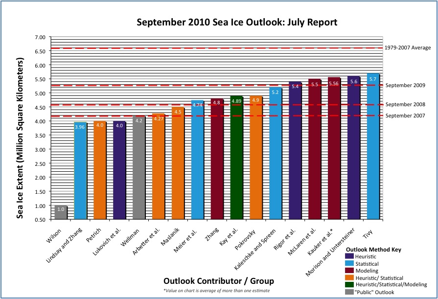
Including all contributors, the individual Outlook values for September 2010 range from 1.0 to 5.6 million square kilometers, with a mean of 4.6 +/- 1.10 million square kilometers. Excluding the outlier of 1.0 million square kilometers by one of the public contributors gives a range of 4.0 to 5.7 million square kilometers, with a mean of 4.8 +/- 0.62 million square kilometers. This is below the 2009 minimum of 5.4 million square kilometers and just slightly above the 2008 minimum of 4.7 million square kilometers. Only three of the Outlook contributions give a value equal to or above the long-term linear trend line (5.6 and 5.7 million square kilometers, respectively). All of the estimates remain significantly below the 1979-2007 average of 6.7 million square kilometers, and six estimates indicate a new record minimum.
The spread of Outlook contributions suggests about a 29% chance of reaching a new September sea ice minimum in 2010 and only an 18% chance of an extent greater than the 2009 minimum (or a return to the long-term trend for summer sea ice loss). 53% of the Outlook contributions suggest the September minimum will remain below 5 million square kilometers, representing a continued trend of declining sea ice extent.
 values for September 2010 sea ice extent. Click to enlarge.")
Pan-Arctic Full Outlook
This month, Julienne Stroeve, NSIDC, acted at guest editor for the Pan-Arctic Outlook.
OVERVIEW OF RESULTS
We welcome four new contributors to the July Outlook. We received 17 responses (Figure 1), with most estimates in the range of 4.0 to 5.7 million square kilometers and one additional Outlook estimate of 1.0 million square kilometers. Nine respondents (excluding the 1.0 million square kilometers prediction) estimate a September minimum below 5 million square kilometers, ranging from 4.0 to 4.9 million square kilometers, while six respondents suggest a minimum between 5.2 and 5.7 million square kilometers. The average estimate is 4.8 +/- 0.62 million square kilometers (excluding the estimate of 1 million square kilometers), below the 2009 minimum of 5.4 million square kilometers and just slightly above the 2008 minimum of 4.7 million square kilometers. All estimates remain significantly below the 1979-2007 mean of 6.7 million square kilometers.
There is general consensus for a persistence of anomalously low sea ice extent. The spread of Outlook contributions suggests about a 29% chance of reaching a new September sea ice minimum in 2010 and only an 18% chance of an extent greater than the 2009 minimum (or a return to the long-term trend for summer sea ice loss). 53% of the Outlook contributions suggest the September minimum will remain below 5 million square kilometers, representing a continued trend of declining sea ice extent.
A variety of methods were used to assess the September 2010 ice extent, including: statistical, comparison with previous observations and rates of ice loss, numerical models, or composites of several approaches. Of interest is that the PIOMAS (Pan-Arctic Ice-Ocean Modeling and Assimilation System) model continues to indicate that the ice is very thin, leading Lindsay and Zhang to predict a new record low for September 2010 with an R2 value of 0.84, suggesting a high degree of skill in the forecast. The numerical modeling methods of Kauker et al. and McLaren et al., however, predict a return to September 2009 conditions, based in part on the presence of older and thicker ice in the East Siberian Sea.
Field observations summarized in the contribution by Hutchings and discussed in this month's Regional Outlook indicate that starting ice thicknesses were comparable to last year in the Beaufort and Chukchi Seas, and that after getting off to a fast start, melt has slowed down considerably, resulting in below-normal melt rates. Buoys show this ice moving into the East Siberian Sea, lending some support to the notion of thicker, more enduring ice in this region.
A lot will depend on the persistence of the low pressure over the central Arctic Ocean. Ice divergence has spread the ice out, slowing the decline in sea ice extent during the first two weeks of July. Yet at the same time, this ice divergence is starting to create openings in the ice pack that readily absorb solar energy, which can lead to more melt. If the ice is as thin as the PIOMAS model suggests, the rate of ice loss is likely to speed up considerably in the next couple of weeks (see the NSIDC Sea Ice News & Analysis for daily updates of ice images).
JUNE 2010 ICE AND ATMOSPHERIC CONDITIONS
After above-average air temperatures and record ice loss in May 2010, the ice extent at the beginning of June fell below the previous record minimum for the same day in 2006. Ice loss during June continued at a fast pace (Figure 2), the fastest rate observed during the month of June in the satellite data record (1979-present), resulting in a new record low sea ice extent in June 2010. According to the National Snow and Ice Data Center (NSIDC), the monthly average June 2010 ice extent was 10.87 million square kilometers, 1.29 million square kilometers below climatology (1979-2000) and 190,000 square kilometers below the previous record low for the month of 11.06 million square kilometers set in 2006. Rapid retreat of the ice cover in the Kara Sea and early melt out of Hudson Bay contributed to this new record low.
.")
Although ice extent at the end of June 2010 was slightly lower than that observed in 2007 (Figure 2), the persistence of the Arctic Dipole Anomaly (DA) throughout the summer of 2007 resulted in an acceleration of ice loss in July that led to the record low ice extent in September 2007. In May and June 2010, the DA was present again, helping to speed up ice loss by promoting clear skies, advection of warm air into the Arctic, and strong offshore winds that move ice away from the coasts. However, in July the sea level pressure (SLP) pattern shifted back to a more typical low pressure region over the central Arctic Ocean (Figure 3), causing ice divergence that has significantly slowed ice loss during the first two weeks of July (Figure 2). This shift is an early repeat of last year.
 for July 1-19 showing low SLP over the central Arctic Ocean, a pattern that brought cooler and cloudier conditions.")
From July 1-July 20, the rate of ice loss averaged -79,810 square kilometers per day. This is a decrease from the average rate of ice loss for June 2010 of -85,210 square kilometers per day, and is slower than climatology (average of -84,050 square kilometers per day for 1979-2000). In the Beaufort Sea, there was little change in ice extent during the first 20 days of July, whereas other regions continued to experience ice loss. Field observations (see Hutchings’ contribution) suggest that clear sky conditions during nighttime may have promoted overnight ice growth on leads and melt ponds, slowing down ice melt. Field observations and a drifting buoy tracking through the region also reveal that widespread refreezing of surface ice meltwater as it comes into contact with colder, more saline seawater, has added ice layers to the bottom of floes, slowing down thinning and melt of the ice cover. Ice extent remains below normal everywhere in the Arctic (Figure 4), with open water developing along the coasts of northwest Canada, Alaska, and Siberia and within the ice pack in the Beaufort Sea and near the North Pole (Figure 5).
 in orange.")
. Note open water developing off Siberian and North American coastlines, and areas of low ice concentration in the central Arctic for the same day as seen in visible-range MODIS imagery (right panel, NASA MODIS Rapid Response System).")
Comparing the latest ice age data from Maslanik and Fowler (see Maslanik contribution) for 21 June 2010 (Figure 6) to current (20 July) ice extent data shows that the ice edge has retreated back to the boundary between first-year and multi-year ice pack in the eastern Arctic and in the Beaufort and Chukchi seas. This has likely delayed further ice loss in these areas, which together with the low SLP over the central Arctic Ocean, accounts in part for the recent decrease in the rate of ice loss seen in Figure 2. Ice remains extensive in the East Siberian and Laptev seas, consistent with wind patterns that favored westward and southward drift into those areas during June. There was virtually no ice loss during June in the East Siberian Sea and ice loss in the Laptev Sea remained slower than normal (Figure 7). However, the low SLP in the central Arctic during the first two weeks of July set up more northward drift along with warm air transport in the East Siberian and Laptev seas, leading to acceleration in ice loss. In July, ice loss in the East Siberian Sea averaged 8,000 sq-km per day between 1-20 July, whereas that in the Laptev and Kara seas averaged -11,260 and -17,110 square kilometers per day, respectively, during the same time period. If the low SLP in the central Arctic persists, we can expect to see rapid retreat of ice in these regions as well as in the Canada Basin. We still anticipate some retreat of the second-year ice (light blue in Figure 6) in the central Arctic and persistence of the older ice into late summer.
 for 21 June 2010. Note a 40% concentration cutoff is used in the ice age maps, which means that ice still could be present in areas shown as 'open water (OW)'.")
.")
KEY STATEMENTS FROM INDIVIDUAL OUTLOOKS
Name (Organization of First Author); Estimate in Million Square Kilometers; Method
Ordered from Greatest to Least Extent
Definitions of the different types of methods can be found in our Sea Ice Outlook glossary. PDFs of the individual contributions are at the bottom of this page.
Tivy (University of Alaska Fairbanks); 5.7 Million Square Kilometers; Statistical
Prediction is unchanged from the June value. The method is based on a simple regression where the predictor is the previous summer (May/June/July) sea surface temperature (SST) in the North Atlantic and North Pacific oceans near the marginal ice zone. Warmer than normal SST is associated with a reduction in ice extent; colder than normal SST is associated with an increase in ice extent.
Morison and Untersteiner (University of Washington); 5.6 Million Square Kilometers; Heuristic
Estimate is based on recent observations, including the previous winter Arctic Oscillation (AO), ice concentrations observed during North Pole Environmental Observatory (NPEO) hydro surveys, atmospheric and ice surface conditions observed with NPEO buoys and Web Cams, and recent ice trajectories. July estimate represents an increase from the previous June estimate of 5.3 million square kilometers.
Kauker et al. (Alfred Wegener Institute for Polar and Marine Research); 5.56 Million Square Kilometers; Numerical Modeling
Note: This value is an average of two estimates:
The ensemble I mean value is 5.78 million square kilometers (bias included) +/- 0.37 million sq kilometers.
The ensemble II mean value is 5.33 +/- 0.37 million square kilometers.
With respect to the June Outlook, the July prediction has increased slightly (about 0.2 million square kilometers). In previous analyses the importance of the initial ice thickness distribution for the ensemble prediction was shown. A comparison of the modeled ice thickness on 1 July 2007, 2008, and 2009, and the initial ice thickness on 26 June 2010 reveals, as for the June Outlook, considerably larger ice thickness mainly in the East Siberian Sea, north of the East Siberian Sea, and in the vicinity of the North Pole in 2010 compared to the years 2007 to 2009. The 'observed' ice concentration on 25 June 2010 shows still a large ice concentration in the areas where large ice thicknesses are modeled, i.e., there is no obvious contradiction between the two fields.
McLaren et al. (Met Office Hadley Centre); 5.5 Million Square Kilometers; Modeling
Prediction is based on an experimental model prediction from the Met Office Hadley Centre seasonal forecasting system (GloSea4) that became operational in September 2009. The September 2010 prediction uses the ensemble mean from 42 runs (3 different start dates each used for 14 runs with different perturbed physics) starting in May.
Rigor et al. (Polar Science Center, University of Washington); 5.4 Million Square Kilometers, Heuristic
The July outlook value is unchanged from the June value. Like last month, the estimate is based on prior winter Arctic Oscillation (AO) conditions and the spatial distribution of ice of different age classes. The June outlook reflects the fact that winds during the last two weeks have reversed the flow of the buoys and sea ice in the Beaufort Gyre and Transpolar Drift Stream, slowing export and sequestering sea ice in the Arctic.
Kaleschke and Spreen (University of Hamburg); 5.2 + 0.1 Million Square Kilometers; Statistical
Estimate is based on AMSR-E sea ice concentrations that are regressed against previous years’ September mean ice extent. Improvements were made to the statistical method, including the use of high resolution AMSR-E sea ice concentration data, a time-domain filter of five days that reduces observational noise, and a space-domain selection that neglects the outer seasonal ice zones. The July outlook is an increase from the June outlook of 4.7 million square kilometers.
Pokrovsky (Main Geophysical Observatory, Russia); 4.9 Million Square Kilometers; Heuristic and Statistical
September sea ice extent is predicted through analysis of three climate indicators: the Atlantic Multidecadal Oscillation (AMO), Pacific Decadal Oscillation (PDO), and Arctic Oscillation (AO) for the last 30 years. Circulation fields for May through June resulted in hot air masses from south Asia and Africa entering Siberia and the Russian Arctic, as well as increasing sea surface temperatures (SSTs) in the North-East Atlantic domain, subjecting the relatively thin ice cover to rapid melting.
Kay et al. (National Center for Atmospheric Research); 4.89 + 0.5 Million Square Kilometers, range of 4.0 to 5.8 million sq kilometers; Heuristic, Statistical, Modeling
Method is an informal inquiry of 19 climate scientists on June 1, 2010. Discussion has focused on the vulnerability of the ice pack from long-term thinning, this year's strong negative winter Arctic Oscillation (AO) state and its influence on ice export and winter temperatures, the fast pace of ice loss in May 2010, and the importance of the unpredictable summer weather conditions.
Zhang (Polar Science Center, University of Washington); 4.8 million Square Kilometers; Modeling
Estimate is based on ensemble predictions starting on July 1, 2010. The ensemble predictions are based on a synthesis of a model, NCEP/NCAR reanalysis data, and satellite ice concentration data. The prediction indicates most of the Northwest Passage will be ice free except for some thin ice in the Lancaster Sound. The revised prediction is a slight increase from the June prediction of 4.7 million square kilometers.
Meier et al. (National Snow and Ice Data Center); 4.74 Million Square Kilometers; Statistical
Prediction by Stroeve et al. shown in the June outlook remains unchanged since it was based on spring ice age fields and an average summer circulation pattern. An alternative method is based on daily rates of decline from July 1 until the minimum is reached. Using average rates of decline based on data from 1979-2000 gives a minimum extent to be significantly lower than the 5.5 million square kilometers earlier forecasted by Stroeve et al.
Maslanik (University of Colorado); 4.5 Million Square Kilometers with possibility of 3.8 Million Square Kilometers; Heuristic/Statistical
Projection is unchanged from the June prediction. Prediction is based on evaluation of ice age that shows current ice extent has retreated back to the multiyear ice edge in the eastern Arctic and in the Beaufort and Chukchi seas. In July, low pressure has become dominant in the central Arctic, which could set up northward drift along with warm air transport in those areas, resulting in rapid retreat of the first-year ice cover in the Siberian seas and Canada Basin. Thick multi-year ice is likely to persist in the southern Beaufort and eastern Chukchi seas.
Arbetter et al. (National Ice Center); 4.27 Million Square Kilometers; Statistical/Heuristic
The most recent data available, week 25 (8 weeks later than the previous forecast) indicates a reduction from the June estimate of 4.85 million square kilometers. The forecast is based on NASA Team sea ice concentrations, NCEP 2-meter air temperature, and NCEP sea level pressure (SLP) as predictors. The estimate is a low bias for prediction versus actual because the area in the Canadian Arctic Archipelago (CAA) is not accounted for.
Lukovich et al. (University of Manitoba); 4.0 Million Square Kilometers; Heuristic
Surface, stratospheric, and ice conditions in 2010 relative to 2007 atmospheric and ice conditions during June provide the basis for projection of September sea ice extent. Similarity in the surface air temperature (SAT) and sea level pressure (SLP) fields in June 2007 and 2010 indicate that sea ice decline will exceed the 2007 record minimum in ice extent. Differences in wintertime stratospheric dynamical phenomena in late winter between 2007 and 2010 suggest that dynamic contributions to ice loss will not be as significant in September 2010 as in 2007. Further investigation of ice thickness and free ice drift conditions, in addition to persistence of SLP maxima, will provide further insight as to whether convergence (divergence) of sea ice associated with SLP highs (lows) will give rise to increased ice retreat in the Arctic and the Beaufort Sea region in particular.
Petrich (University of Alaska Fairbanks); 4.0 Million Square Kilometers, with a possible range of 3.4 to 5.4 million square kilometers, likely range of 3.4 to 4.9 million square kilometers; Heuristic, Statistical
June sea level pressure (SLP) is related to both surface winds and clouds, which are known to drive arctic sea ice reduction in summer. The mean June SLP is used as a proxy for September sea ice extent because the association appears to be stronger than for any other month.
Lindsay and Zhang (Applied Physics Laboratory, University of Washington); 3.96 + 0.34 Million Square Kilometers; Statistical PIOMAS
Model results indicate the ice has continued to thin at a fast rate. The best predictors for the September minimum are G1.0 (area with less than 1.0m of ice) and G0.4 (area with less than 0.4m of ice), both of which give nearly identical results. Using the G1.0 predictor that was used in the June outlook gives a prediction of 3.96 +/- 0.34 million square kilometers, with an R2 value of 0.84, indicating a high degree of skill in the forecast. This is a decrease from the June outlook prediction of 4.4 million square kilometers.
Public Contributions:
Wellman (no organization provided); 4.2 Million Square Kilometers; Statistical
A linear fit between spring/early summer PIOMAS volume anomaly for each year from 2000-2009 against the September minimum yields a 2010 estimate of 4.2 million square kilometers, a decrease from the previous estimate of 5.1 million square kilometers.
Wilson (no organization provided); 1 million Square Kilometers; Statistical and Heuristic
Prediction is that the El Nino of 2010 will result in rapid ice melt. With the end of the El Nino cycle and the beginning of a La Nina, prediction is that skies will become clearer, resulting in more surface melt that is further enhanced by the ice-albedo feedback.
| Attachment | Size |
|---|---|
| Combined Individual Outlook Contributions13.78 MB | 13.78 MB |
| Attachment | Size |
|---|---|
| Tivy28.47 KB | 28.47 KB |
| Morison and Untersteiner26.78 KB | 26.78 KB |
| Kauker et al.683.05 KB | 683.05 KB |
| McLaren et al.196.56 KB | 196.56 KB |
| Rigor et al.4.88 MB | 4.88 MB |
| Kaleschke and Spreen1.8 MB | 1.8 MB |
| Pokrovsky253.1 KB | 253.1 KB |
| Kay et al.37.6 KB | 37.6 KB |
| Zhang77.75 KB | 77.75 KB |
| Meier et al.231.6 KB | 231.6 KB |
| Maslanik65.96 KB | 65.96 KB |
| Arbetter et al.382.83 KB | 382.83 KB |
| Lukovich et al.2.98 MB | 2.98 MB |
| Petrich36.31 KB | 36.31 KB |
| Lindsay and Zhang711.94 KB | 711.94 KB |
| Public Contribution - Wellman83.06 KB | 83.06 KB |
| Public Contribution - Wilson623.2 KB | 623.2 KB |
| Ship Observations - Hutchings177.62 KB | 177.62 KB |
| Attachment | Size |
|---|---|
| Gerland et al.641.93 KB | 641.93 KB |
| Gudmandsen755.25 KB | 755.25 KB |
| Howell and Agnew706.7 KB | 706.7 KB |
| Lindsay and Zhang42 KB | 42 KB |
| Maslanik65.96 KB | 65.96 KB |
| Petrich et al.132.58 KB | 132.58 KB |
| Pokrovsky253.1 KB | 253.1 KB |
| Rigor et al.4.88 MB | 4.88 MB |
| Tivy180.15 KB | 180.15 KB |
| Zhang87.62 KB | 87.62 KB |
| Ship Observations - Hutchings177.62 KB | 177.62 KB |
 values for September 2010 sea ice extent. Click to enlarge.")