
Outlook Report
Executive Summary
Thank you to the groups that contributed to the 2016 June report. We received 30 contributions that include pan-Arctic predictions and two additional contributions with a regional focus.
This June Outlook report was developed by lead authors, Julienne Stroeve (NSIDC) and Ed Blanchard-Wrigglesworth (UW), with contributions from the rest of the SIPN Leadership Team.
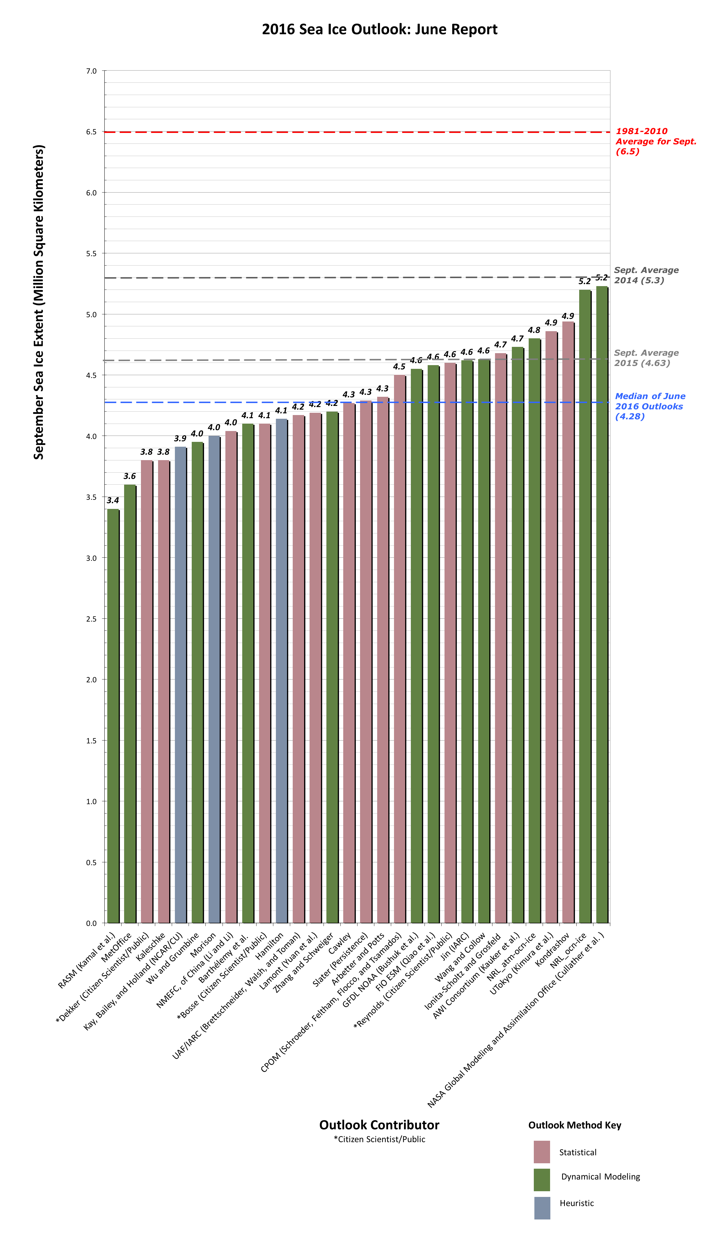
The median Outlook value for September 2016 sea ice extent is 4.28 million square kilometers with quartiles of 4.10 and 4.63 million square kilometers (See Figure 1 in the full report, below). Contributions are based on a range of methods: statistical, dynamical models, estimates based on trends, and two informal polls. This year the spread in the Outlook contributions is not as large as last year: the overall range is 3.40 to 5.23 million square kilometers, compared to last year's spread of 3.3 to 5.7 million square kilometers. The median Outlook value is also down from last year by more than 700,000 square kilometers. This year's forecast compares to observed values of 4.3 million square kilometers in 2007, 3.6 million square kilometers in 2012, and 4.63 million square kilometers in 2015. Only one forecast suggests a new record low is possible, one ties with 2012, while all others do not forecast a new record low for 2016.
A discussion of 13 dynamical model contributions shows that the variance among the individual outlooks is substantially less than last year and as a whole. For all 13 dynamical models, the median prediction is 4.58 million square kilometers, with quartiles of 4.10 and 4.73 million square kilometers. This is compared to the statistical contributions that show a slightly smaller median extent of 4.28 million square kilometers (quartiles of 4.11 and 4.58 million square kilometers).
A section on predicted spatial fields includes discussion on sea ice probability (SIP) and the first ice-free day (IFD) from a number of dynamical models. Finally, a section on current conditions includes discussion of this spring's record low sea ice conditions, observations of sea ice thickness, and atmospheric conditions.
(Please note: The Sea Ice Outlook provides an open process for those interested in Arctic sea ice to share predictions and ideas; the Outlook is not an operational forecast.)
Overview
The Outlook contributions this June are based on a range of methods: statistical, dynamical models, estimates based on trends, and subjective information. Since 2008 when the SIO started, we have seen a shift from less quantitative heuristic methods towards more quantitative contributions based on statistical and dynamical models. This month, we only had 3 heuristic contributions (two from informal polls), 14 contributions using statistical methods (including estimates based on trends) and 13 using dynamical models, 8 of which were fully-coupled climate models. Fully-coupled models simulate all of the major components of the climate system—including ice, ocean, atmosphere, and land—and allow these to vary and interact together within the model, which provides a more complete representation of the complex sea ice system.
The distribution of Outlooks for statistical and dynamical models have a median extent that is 0.15 million square kilometers different from each other, with a slightly larger spread for the statistical models than the dynamical models. The same sort of spread difference was seen in 2015. Separating out fully-coupled dynamical models from ice-ocean models shows that fully coupled models give a slightly lower forecast with a median of 4.57 versus 4.62, yet have a larger spread (Figure 2). The median forecast of heuristic forecasts is 4.0 million square kilometers and the spread is small. However, actual contributions to the two polls show a diverse range from 2.9 to 5.3 million square kilometers.
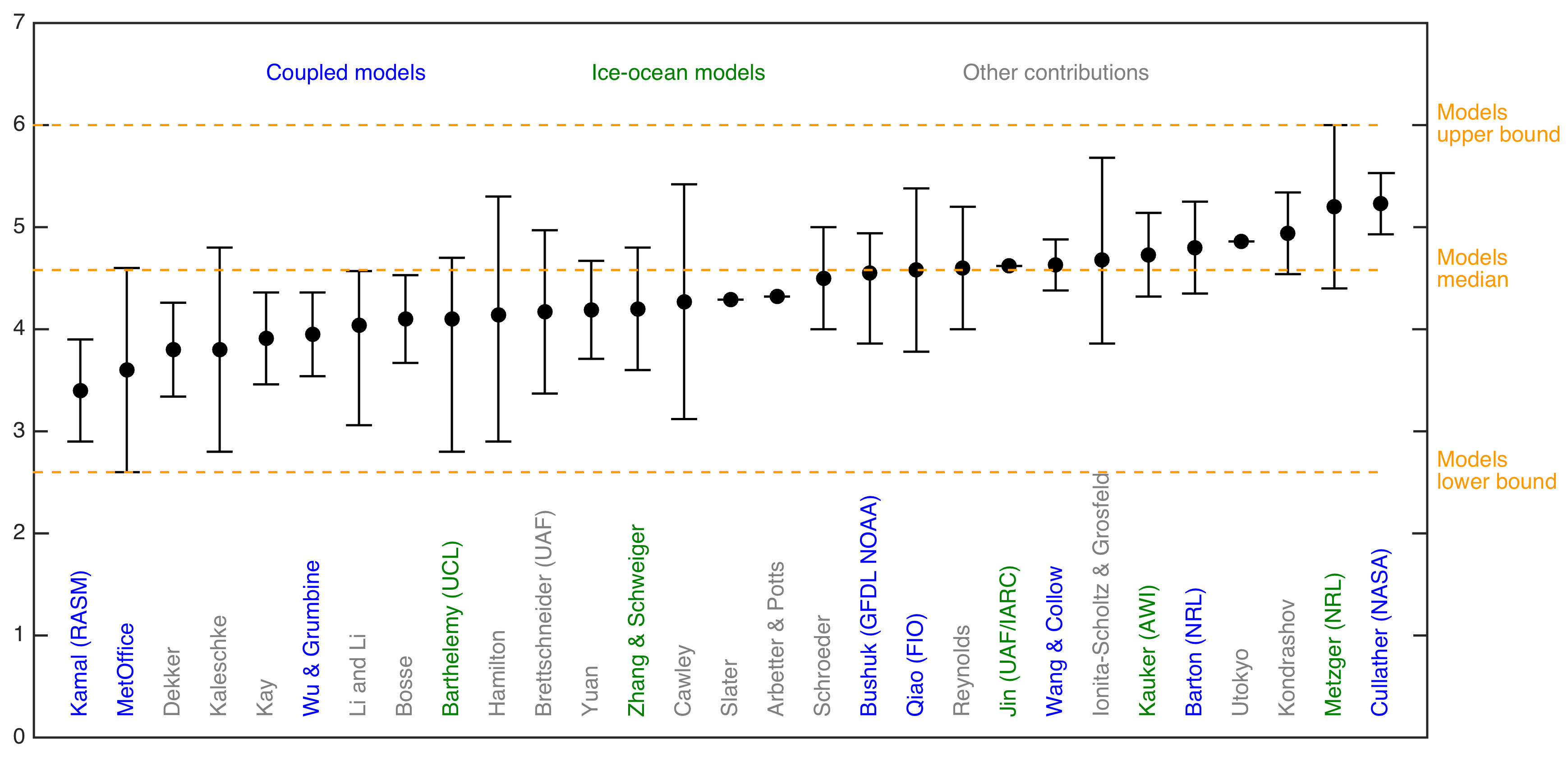
The overall width of the distribution of Outlooks has narrowed compared to last year: the interquartile spread across all types of contributions is 0.53 million square kilometers, which is a decrease of 0.27 million square kilometers since last year. The overall range is also reduced to 3.4 to 5.23 million square kilometers. Note that both extreme ends for this year's forecast range come from fully coupled climate models (RASM/Kamal and NASA/Cullather), as can be seen in Figure 2 by the considerably larger spread than seen for the ice-ocean dynamical models.
 for September 2016 sea ice extent. We do not show submissions that were received late, thus n=30 in this figure and all subsequent figures.")
Download a high-resolution version of Figure 1.

Comment On Dynamical Modeling Contributions
2016 Modeling Contributions at a Glance
This year we received 13 June SIO submissions from dynamical models, of which 5 were from ice-ocean models forced by atmospheric reanalysis or other atmospheric model output (in green in Figure 3) and 8 were from fully-coupled general circulation models (in blue in Figure 3). The median extent predicted by the models this year is 4. 58 million square kilometers (mean: 4.43 million square kilometers), which is lower than last year's median for the June report of 5.07 million square kilometers (mean: 5.05 million square kilometers).
Decomposition of the Spread in the 2015 Model Predictions
The spread among individual model outlooks (the dots in Figure 3) amounts to 0.56 million square kilometers, which is similar to the spread among model outlooks seen in previous years. Assuming that the number of ensemble members used to produce the individual model submissions is large enough, each outlook averages away the unpredictable noise due to the atmosphere. In other words, the standard deviation of 0.56 million square kilometers captures the uncertainty associated with factors that can (hopefully) be controlled and reduced in the future: initial conditions, resolution, and model errors. The remainder of total spread is associated with the unpredictable, chaotic evolution of the atmosphere between June and September, and is represented by the error bars in Figure 3. We estimate that this uncertainty due to chaos amounts to a model-mean of 0.58 million square kilometers (i.e., the mean of all models' submissions error bars in Figure 3). Thus, both irreducible errors and differences in model configurations and initial conditions contribute comparably to forecast uncertainty.
 and from all other methods (grey). The dots are the outlook themselves and the intervals are the uncertainty ranges provided by the groups. Definitions of uncertainty were left to the discretion of the groups themselves, and should therefore be compared with caution. The middle dashed horizontal line is the median of the outlooks from dynamical modeling groups. The lower (upper) dashed horizontal line is the lowest (largest) bound when all dynamical modeling contributions are considered. Image courtesy of Edward Blanchard-Wrigglesworth.")
Download a high-resolution version of Figure 3.
Comment On Predicted Spatial Fields
As we did in the last two years, we have requested contributions of sea ice probability (SIP) and first ice-free date (IFD). SIP is defined as the fraction of ensemble members in an ensemble forecast with September ice concentration in excess of 15%. IFD is the date in the melt season at which the ice concentration at a given location first drops below 15%. So far this year, we have received 6 submissions of SIP and 3 of IFD.
 from 6 dynamical models, the mean of all 6, and the standard deviation across all 6 SIP forecasts. NRL FC corresponds to Barton (NRL) and NRL IO to Metzger (NRL) in Figure 3.")
The models that forecast lower extent in Figure 3 (e.g., MetOffice) tend to forecast lower SIPs, and vice versa. While there is some spread in the SIP forecasts, it is interesting to note that forecasts agree better in the European sector (northern Svalbard/Barents/Kara) relative to the East Siberian/Alaskan sectors, as shown by the across-model standard deviation in the SIP forecast (last panel in Figure 4).
The forecasts of IFD are shown in Figure 5. As in past summers, there is considerable spread across models' forecasts, with NASA (Cullather et al) having rather late IFDs compared to both NRL forecasts (Barton and Metzger).
 from 3 dynamical models. NRL FC corresponds to Barton (NRL) and NRL IO to Metzger (NRL) in Figure 3. Image courtesy of Edward Blanchard-Wrigglesworth.")
Current Conditions
Winter 2016 in the Arctic set several records, including record warmth in December, January, and February (DJF warmest since 1880), and subsequently record low sea ice extents in January, February, and March, as well as the lowest maximum extent recorded thus far since the satellite observations began. This record low followed on the previous record low winter maximum observed last year. Part of the explanation for the record winter warmth and reduced ice growth comes from a large Arctic cyclone at the end of December 2015 that brought warm and humid air into the Arctic, particularly over the Kara and Barents seas that contributed to the record low ice conditions in January and February. Above freezing conditions were also observed at the North Pole during December. In January and February there were southerly winds blowing across Alaska that contributed to a second Arctic temperature maximum, termed the "split vortex" by Overland and Wang (2016). Based on different reanalysis products, Arctic-wide (averaged over 66˚-90˚N) temperatures for both January and February were more than 3-6 ˚C warmer than the previous record value.
Airborne sea ice thickness surveys over the Canadian Arctic Archipelago and the southern Beaufort Sea revealed that multiyear ice thickness was generally similar to that observed in 2015, but that the first-year ice was thinner (< 2m), likely a result of the unusually warm winter that limited growth of first-year ice (Figure 6). The thickness surveys and visible imagery also revealed a fragmented ice cover in the Beaufort Sea as a result of wind-driven ice divergence, making this region particularly vulnerable to melting out during summer (Figure 7). This region showed early development of open water that contributed towards the record low May sea ice extent. Near Barrow, Alaska, thickness surveys from IceBridge (Figure 8) suggest areas of thin ice, which is confirmed from Barrow Ice Mass Balance (IMB) buoys. Landfast ice never exceeded 1m this year at Barrow, which appears to be a result of reduced winter ice growth and early melt onset in April.
 (left) and first-year ice (FYI) regimes (right) in the Beaufort Sea for the individual, eastern, and western surveys in 2016, and combined histograms for both flights in 2015. Figure courtesy C. Haas, York University.")
 sensor in the Beaufort Sea on April 9 and 10, 2016, superimposed on concurrent imagery from the Moderate Resolution Imaging Spectroradiometer (MODIS) sensor on the NASA Terra and Aqua satellites. Figure courtesy C. Haas, York University.")

As a result of anomalously mild winter ice conditions combined with warmer than average air temperatures, sea ice in May also reached a new record low, more than 1 million square kilometers below any previous May in the satellite record (since 1979). The mild ice conditions were dominated by lower than average ice concentration/extent in the Kara, Barents, and East Greenland seas on the Eurasian side, the Chukchi Sea and early opening of the ice pack in the southern Beaufort Sea on the Pacific side (Figure 9). Many SIO contributors assimilate conditions in May in their forecasts, which likely explains why this year's forecasts were considerably lower than last year. However, despite starting out the melt season with significantly less sea ice than observed in 2012, colder than normal conditions for June, linked to lower than normal sea level pressure, (Figures 10 and 11) slowed the ice loss and the ice extent currently is neck-and-neck with that observed in 2012, the year with the record low sea ice extent. As of June 21, 2016, the 2016 sea ice extent is 10.2 million square kilometers, compared to 10.33 in 2012.
Low sea level pressures are historically not associated with extreme sea ice summer minima. This weather pattern is expected to continue through the first half of July; the National Weather Service 500 mb outlook shows support for the same pattern of lower pressures in the Beaufort Sea and higher pressures in the Barents and Kara Seas (Figure 12).
 and daily sea ice extent from March through June 19 2016 for 2016 (blue), 2012 (green) and the 1981-2010 long-term mean (black) and 2 standard deviations (gray shading). Credit: NSIDC.")


Key Statements/Executive Summaries From Individual Outlooks
The Outlooks are listed below in order of lowest to highest predicted September extent. Extent and uncertainty (in parentheses) values are provided below in units of millions of km2 unless noted otherwise. The individual outlooks can be downloaded as PDFs at the bottom of this webpage.
RASM (Kamal et al.), 3.4 (±0.5), Modeling (fully-coupled)
Sea ice extent (i) monthly average annual cycle was calculated for 1988-2014 and (ii) trend for 1996-2014 both from Regional Arctic Climate Model (RASM) simulation and from NSIDC Merged SMMR and SSM/I sea ice concentration data. Model residual monthly ice extents were calculated by removing modal monthly average annual cycle and model linear trend. These residuals carry only information about the model hindcasted or predicted inter-annual variability. To correct for the known model biases we added to these model residuals the observed monthly average annual cycle and observed linear trend to estimate biases corrected monthly ice extents from 1996 through September 2016. Bias between the observed values and those from RASM after statistical correction from 1996 to 2014 is trendless and is used to estimate uncertainty in the September 2016 prediction.
Met Office, 3.6 (±1.0), Modeling (fully-coupled)
Using the Met Office GloSea5 seasonal forecast systems we are issuing a model based mean September sea ice extent outlook of 3.6 ± 1.0 million km2. This has been assembled using start dates between 15 May and 4 June to generate an ensemble of 42 members.
Dekker (Citizen Scientist/Public)*, 3.8 (Std dev = 0.46), Statistical
For this projection, I used the monthly May snow cover data from the Rutgers Snow Lab, as well as the NSIDC monthly Extent-minus-Area (as a metric to estimate the presence of open water such as leads and melt ponds), over the 1992-2015 period known September extent data. This method is based on the physics of albedo amplification during summer, and obtains a 0.46 million km2 standard deviation in the prediction, which is better than most other methods, albeit not that much better than a simple "linear trend" prediction. The important finding is that spring snow cover signal is clearly present in the September Arctic sea ice extent.
Kaleschke, 3.8 (±1.0), Statistical
I provide a simple statistical estimate for the September sea ice extent based on the total sea ice extent measured on June 11: 3.8±1.0 million km2. For regular updates of the graphs follow me on Twitter @seaice_de.
Kay, Bailey, and Holland (NCAR/CU), 3.91 (Std dev = 0.45), Heuristic
An informal pool of 27 climate scientists in early June 2016 estimates that the September 2016 ice extent will be 3.91 million km2. (stddev. 0.45, min. 3.14, max. 4.80). Since its inception in 2008, the NCAR/CU sea ice pool has easily rivaled much more sophisticated efforts based on statistical methods and physical models to predict the September monthly mean Arctic sea ice extent (e.g. see appendix of Stroeve et al. 2014 in GRL doi:10.1002/2014GL059388 ; Witness the Arctic article by Hamilton et al. 2014). We think our informal pool provides a useful benchmark and reality check for Sea Ice Prediction efforts based on more sophisticated physical models and statistical techniques.
Wu and Grumbine, 3.95 (Std dev = 0.41), Modeling (fully-coupled)
The projected Arctic minimum sea ice extent from the NCEP CFSv2 model with revised CFSv2 May initial conditions (ICs) using 31-member ensemble forecast is 3.95 million km2with a standard deviation (SD) of 0.41 million square kilometers. The Minimum and Maximum values for the Arctic sea ice extent in the 31-member ensemble prediction are 3.35 and 4.89 million km2, respectively.
Morison, 4.0, Heuristic
I had conversations with Axel Schweiger and others following the Seasonal Ice Zone Reconnaissance Surveys (SIZRS) flights during third week of June 2016, who observed some melting but no big ponds as yet. There was open water on and south of 150W, 72N, which puts the ice retreat edge a bit earlier than seen recently. Ice was solid from 74N to 75N with more leads at 76 N, which seems similar to early season patterns seen in recent years that have and intermediate region of pretty solid conditions somewhere south of the Beaufort Gyre center. Usually more winter snow in the Central Arctic has seemed to indicate less September sea ice extent. But, with no spring observations from the North Pole Environmental Observatory in the central Arctic ocean in 2016 I don’t know what the snow conditions were like in that region this year. The winter Arctic Oscillation index was about the same as for 2011 and a similar deviation below the long- term tend would suggest a 2016 minimum extent of 4.2 million sq. km. This is pretty squishy, but given the current extent and ice conditions in the Beaufort Sea, I think this year’s September average will be about 4 million sq. km.
NMEFC, of China (Li and Li), 4.04 (3.06-4.57), Statistical
We predict the September monthly average sea ice extent of Arctic by statistic method and based on monthly sea ice concentration and extent from National Snow and Ice Data Center. The result shows that the Sep. ice extent of 2016 will be less than in 2015.
Barthélemy et al., 4.1 (2.8-4.7), Modeling (ice-ocean)
Our estimate is based on results from ensemble runs with the global ocean-sea ice coupled model NEMO-LIM3. Each member is initialized from a reference run on May 31, 2016, then forced with the NCEP/NCAR atmospheric reanalysis from one year between 2006 to 2015. Our final estimate is the ensemble median, and the given range corresponds to the lowest and highest extents in the ensemble.
Bosse (Citizen Scientist/Public), 4.1 (±0.43), Statistical
Just as in the two years before I calculate the value for the September-minimum of the arctic sea ice extent of the year n (NSIDC monthly mean for September) from the Ocean Heat Content (0…700m depth) northward 65°N during JJAS of the year n-1. After 2006 the lower sea ice volume of the Februaries also impacts the minimum extent. For the physical explanation see https://www.arcus.org/files/sio/23220/bosse_july2015.pdf .
Hamilton, 4.14 (2.9-5.3), Heuristic
At the Polar Prediction Workshop in May, we carried out an informal poll asking participants for their personal guess about the extent of Arctic sea ice in September 2016. Thirty-five people responded with answers ranging from 2.9 to 5.3 million km2 (see Figure 1 in contribution). The lowest prediction would set a new historical record, far below the previous low point of 3.62 set in 2012. The highest prediction would simply mark a return to the 2014 level, which is well below any observations before 2007. So no one is expecting an Arctic sea ice “recovery.” The average among these 35 informal predictions is 4.14 19 million km2, which would make September 2016 the second-lowest extent we have seen.
UAF/IARC (Brettschneider, Walsh, and Thoman), 4.17 (±0.8), Statistical
The outlook is based on an objective analog methodology designed to predict the summer atmospheric fields that drive sea ice variations. The analog years are the ones in which atmospheric circulation and temperature fields best match those of 2016 through May. The actual forecast ice extent is the mean of the September ice extent in the five best analog years of the past (from 1979-2015).
Lamont (Yuan et al.), 4.19 (±0.48), Statistical
A Linear Markov model is used to predict monthly Arctic sea ice concentration at all grid points in the pan Arctic region. The model is a stochastic linear inverse model that is built in the multi-EOF space and is capable to capture the co-variability in the ocean-sea ice-atmosphere system. September pan Arctic sea ice extent is calculated from predicted sea ice concentration. The model predicts that large negative sea ice concentration anomalies (< -40%) will occur in the Beaufort Sea, Chukchi Sea, Laptev Sea, Kara Sea and Barents Sea in September 2016. The September mean total Arctic sea ice extent will be 4.19 million km2.
Zhang and Schweiger, 4.2 (±0.6), Modeling (ice-ocean)
Driven by the NCEP CFS forecast atmospheric forcing, PIOMAS is used to predict the total September 2016 Arctic sea ice extent as well as ice thickness field and ice edge location, starting on June 1. The predicted September ice extent is 4.2± 0.6 million km2. The predicted ice thickness fields and ice edge locations for June–August 2016 are also presented.
Cawley, 4.27 (±1.15), Statistical
This is a purely statistical method (Gaussian Process, related to Kriging) to estimate the long-term trend from previous observations of September Arctic sea ice extent. As this uses only September observations, the prediction is not altered by observations made during the Summer of 2016.
Slater (Persistence), 4.29 (Avg of 4.88, 4.96, and 3.03), Statistical
Persistence can be computed in several ways. I have looked out to September for the sake of comparison and as a very basic benchmark.
1) Daily anomaly persistence at 112 days lead time (so that I can go all the way to Sep 30th), then compute mean for Sept = 4.88 million km2
2) Persist the absolute anomaly from May to Sept (using NSIDC monthly value, not mean of daily). Sept = 4.96 million km2
3) Persist the standard normal deviate from May to Sept (using NSIDC monthly). Labeled as "Variance Persistence". Sept = 3.03 million km2
None of these methods have true skill at this long lead time. For April-June the daily persistence at 112-day lead time looks like a nice forecast (and is giving better results than a 50-day lead time), however, this is pure coincidence. These methods are different from the “damped persistence” that Ed Blanchard-Wrigglesworth calculates (as I have no damping mechanism built in).
Arbetter and Potts, 4.32 (based on 10 June data), Statistical
This method is based on the Arctic Regional Ice Forecast System (Drobot et al., International Journal of Climatology, 2009) with additional modifications done by Arbetter at National Ice Center; followed by rewriting and parallelizing the code done by Potts. It uses sea ice, sea level pressure (NCEP), 2-meter surface air temperature (NCEP), and cumulative freezing degree days. Ten years of data are used to establish correlations between conditions at the start week and forecast week. Forecasts are done for 12-16 weeks in the future to cover melt and refreezing.
CPOM (Schroeder, Feltham, Flocco, and Tsamados), 4.5 (±0.50), Statistical
We predict the September ice extent 2016 to be slightly lower than last year. Given the extreme low current sea ice extent and the positive SST anomalies, a stronger decline might be expected. But looking at the May 2016 melt pond fraction in our sea ice simulation, the pond fraction is higher in the Kara Sea, north of Svalbard and in the Fram Strait compared to May 2015 and with a lesser extent to May 2012, but lower in the East Siberian Sea and the Arctic Basin. The weighted Arctic wide mean May pond fraction 2016 is higher than in 2015, but much lower than in 2012. While the ice thickness is generally thinner in May 2016 compared to previous years, the air temperature has been several degrees above the last 10 year mean in the northern North Atlantic and the Beaufort Sea, but colder in the Eastern Siberian Sea and Laptev Sea causing the described melt pond pattern.
GFDL NOAA (Bushuk et al.), 4.55 (3.86-4.94), Modeling (fully-coupled)
Our June 1 prediction for the September-averaged Arctic sea-ice extent is 4.55 million km2, with an uncertainty range of 3.86-4.94 million km2. Our prediction is based on the GFDL-FLOR ensemble forecast system, which is a fully-coupled atmosphere-land-ocean-sea ice model initialized using a coupled data assimilation system. Our prediction is the bias-corrected ensemble mean, and the uncertainty range reflects the lowest and highest sea ice extents in the 12-member ensemble.
FIO ESM (Qiao et al.), 4.58 (±0.80), Modeling (fully-coupled)
Our prediction is based on FIO-ESM with data assimilation. The prediction of September pan-Arctic extent in 2016 is 4.58 (+/-0.80) million km2. 4.58 and 0.80 million km2 is the average and one standard deviation of 10 ensemble members, respectively.
Reynolds (Citizen Scientist/Public), 4.6 (±0.6), Statistical
April gridded PIOMAS data is used to calculate the April volume for the Arctic Ocean including Kara, Barents, Greenland Sea and the Canadian Arctic Archipelago. This is then used together with September extent for each year, 1979 to 2015, and a relationship between April volume and September thickness is calculated. The prediction is then based upon April volume for the current year.
Jin (IARC), 4.62, Modeling (ice-ocean)
A coupled ice-ocean model (POP-CICE) forecast of the September sea ice extent minimum. The Model is initialized with PHC data and runs from 1958‐2009 with CORE 2 forcing, 2010-2016 with GFDL IPCC atmospheric model output. Since there is only one run, we cannot provide uncertainties.
Wang and Collow, 4.63 (±0.25), Modeling (fully-coupled)
The contribution here includes (1) Monthly September sea ice extent, (2) Monthly September sea ice extent error estimate, and (3) Date of September minimum. We will try to add other additional/optional items for July and August reports. Used CFSv2pp dynamical model; Twenty ensemble members are used. The ensemble members are generated from 5 initial dates (8th - 12th of May at 00Z) with four runs from each initial date. The four runs from each initial date include a control run initialized from CFSR and three additional runs with perturbed initial conditions.
Ionita-Scholtz and Grosfeld, 4.68 (3.86-5.68), Statistical
Sea ice in both Polar Regions is an important indicator for the expression of global climate change and its polar amplification. Consequently, a broad information interest exists on sea ice, its coverage, variability and long-term change. Knowledge on sea ice requires high quality data on ice extent, thickness and its dynamics. As an institute on polar research we collect data on Arctic and Antarctic sea ice, investigate its physics and role in the climate system and provide model simulations on different time scales. All this data is of interest for science and society. In order to provide insights into the potential development of the seasonal signal, we developed a robust statistical model based on ocean heat content, sea surface temperature and atmospheric variables to calculate an estimate of the September minimum sea ice extent for every year. This is applied for the year 2016 the first time and we will provide updated results every month for the sea ice outlook report.
AWI Consortium (Kauker et al.), 4.73 (±0.41), Modeling (ice-ocean)
Sea ice-ocean model ensemble prediction run initialized with assimilation of sea ice and ocean observations.
NRL_atm-ocn-ice, 4.8 (4.4-5.3), Modeling (fully-coupled)
The projected Arctic minimum sea ice extent from the Navy’s global coupled atmosphere-ocean-ice modeling system is 4.8 million km2. This projection is the average of an 11-member ensemble. The range of the ensemble is 4.4 to 5.3 million km2. Note that our ensemble range does not represent a full measure of uncertainty, and the system is currently in a development stage.
UTokyo (Kimura et al.), 4.86, Statistical
Monthly mean ice extent in September will be about 4.86 million square kilometers. Our estimate is based on a statistical way using data from satellite microwave sensor. We used the ice thickness in December and ice movement from December to April. Predicted ice concentration map from July to September is available in our website: http://ccsr.aori.u-tokyo.ac.jp/~kimura_n/arctic/1st_e.html
On the Russian side, sea ice in the Laptev Sea is expected to retreat quickly. On the other hand, sea ice in the East Siberian Sea is likely to retreat slowly. The ice retreat in the East Siberian Sea will be late compared with the last year because the area is covered by thicker ice piled up by the winter convergence of sea ice. On the Canadian side, sea ice in summer is expected to be thin and retreat more quickly than the last year.
Kondrashov, 4.94 (Std dev = 0.4), Statistical
This contribution relies on data-driven approach to predict sea ice conditions over the Pan-Arctic region. The prediction model is obtained by data-adaptive decomposition and inverse modeling of Multisensor Analyzed Sea Ice Extent – Northern Hemisphere (MASIE-NH) dataset.
NRL_ocn-ice, 5.2 (4.2-6.0), Modeling (ice-ocean)
The Global Ocean Forecast System (GOFS) 3.1 was run in forecast mode without data assimilation, initialized with May 1, 2016 ice/ocean analyses, for ten simulations using National Centers for Environmental Prediction (NCEP) Climate Forecast System Reanalysis (CFSR) atmospheric forcing fields from 2005-2014. The mean ice extent in September, averaged across all ensemble members is our projected ice extent. The GOFS 3.1 outlook for the 2016 September minimum ice extent is 5.2 million km2 with a range of 4.2 – 6.0 million km2.
NASA Global Modeling and Assimilation Office (Cullather et al.), 5.23 ± 3.0, Modeling (fully-coupled)
The GMAO seasonal forecasting system predicts a September average Arctic ice extent of 5.23±0.30 million km2, about 13 percent greater than the 2015 value. While the initial ice cover is remarkably low in the Barents and Kara seas, the forecast suggests limited reductions in ice extent on the Pacific side of the Arctic as compared with recent years. This is the final year of sea ice forecasts with the current system, a new GMAO seasonal forecasting system will be in place next year.
Druckenmiller and Eicken – Regional for Bering-Chukchi-Beaufort Seas
In this contribution, Druckenmiller and Eicken discuss the anomalous spring conditions that have been observed in the Bering-Chukchi-Beaufort (BCB) Region.
Souness – Perspectives on Ice Breaker Impacts
In this contribution, Souness proposes that accounting for icebreaker routings could be beneficial when forecasting the nature and extent of sea ice in certain areas.
Individual Outlook PDFs
