
Outlook Report
Executive Summary
Thank you to the groups that contributed to the 2017 June and July reports. For July we received 36 contributions for pan-Arctic extent predictions. Eight contributed Alaska regional extent predictions, 12 contributed for Antarctica, and two informal contributions were received. This July Outlook report and current conditions was coordinated by lead author James Overland (NOAA) with contributions from Edward Blanchard-Wrigglesworth (University of Washington), François Massonnet (Université Catholique de Louvain and Barcelona Super Computing Center), and the SIPN Leadership Team.
For the July Report there were 36 contributions with the median Arctic Outlook value for September 2017 sea ice extent of 4.5 million square kilometers with quartiles of 4.2 and 4.8 million square kilometers (See Figure 1 in the Overview section, below). These values are 0.1 higher than the June Report, and suggest the impact of moderating summer 2017 Arctic weather. The range is 3.1 to 5.5 million square kilometers. To place this Outlook in context, recently observed values were 4.3 million square kilometers in 2007, 3.6 million square kilometers in 2012, and 4.7 million square kilometers in 2016. Contributions are based on multiple methods: statistical, dynamical models, heuristic, and mixed. In the June Report the largest value was from a model, while the four largest values in July are from statistical methods. Of interest is that the heuristic approach, influenced by initial low May sea ice extents, continues to have the lowest median value among the various methods. Two participants state that a new record low is likely, though several others suggest it is possible; this seems unusual given the record low extents at the start of the season.
The current conditions section highlights that winter 2017 had record low sea ice, but since May sea ice extents are similar to, and slightly above, the previous record from 2012. Atmospheric air temperatures and lower sea level pressures were not favorable for rapid sea ice loss in June and early July 2017. Forecast atmospheric weather conditions continue to be less favorable for major sea ice loss Such low initial sea ice amounts but not unusual summer weather are consistent with the consensus of the July Outlooks for low, but non-necessarily record September sea ice conditions in 2017.
Please note: The Sea Ice Outlook provides an open process for those interested in Arctic sea ice to share predictions and ideas; the Outlook is not an operational forecast.
Overview
Arctic Outlook contributions are based on multiple methods: statistical, dynamical models, estimates based on trends, and subjective information (Figure 1). This July there were 3 heuristic contributions, 3 mixed contributions that rely on a combination of statistical approaches and heuristic assessment, 15 contributions using statistical methods, and 15 using dynamical models. Fully-coupled models simulate all of the major components of the climate system—including ice, ocean, atmosphere, and land—and allow these to vary and interact together within the model.
Summary statistics (median; first and third quartiles) for contributions of each method type are given below (in millions of square kilometers):
| Method Type | Med | Q1 | Q3 |
|---|---|---|---|
| Heuristic | 4.1 | 3.4 | 4.4 |
| Statistical | 4.7 | 4.5 | 5.1 |
| Mixed | 4.2 | 4.0 | 4.6 |
| Dynamical | 4.5 | 4.1 | 4.6 |
| All | 4.5 | 4.2 | 4.8 |
The data set is available here.
 for September 2017 sea ice extent.")
The lowest forecast value comes from a dynamical model that simulates the sea ice coupled to atmosphere and ocean model components, and the second lowest is from a heuristic contribution that considered the amount of multiyear ice over the winter of 2016/2017 together with the mean winter atmospheric circulation pattern. The four highest forecasts are statistical. In June the highest value was a pre-operational model.
The distribution plot of Outlooks by method (Figure 2) shows the heuristic estimates are below the overall median of 4.5 million square km and statistical methods slightly above the overall median. Outlooks from statistical and dynamical models have a considerable range within their respective categories, most likely because there are many more contributions from these methods.

Druckenmiller and Eicken report ice concentration in the Beaufort Sea is well below normal but over 20% greater than the extreme anomalous conditions during 2016. Multi-year ice is low to completely lacking. For the Nares Strait region, Gudmandsen expects variable north/south drift will continue during July and due to increasing surface melting, multiyear floes will be at low concentration by 1 August in the Smith Sound.
Two groups comment on sea ice volume. AWI notes that April 2017 has the third lowest sea ice volume in the CryoSat record. Viddal notes an increase in the annual average sea ice volume drop/year in 2015, 2016 and 2017 compared to prior years based on PIOMAS calculations.
Comments on Predicted Spatial Fields
Again this month we have received a record number of September Sea Ice Probability (SIP) forecasts with 11 groups contributing (Figure 3). SIP is defined as the fraction of ensemble members in an ensemble forecast with September ice concentration in excess of 15%. Nine of the groups that submitted a June SIP forecast submitted a July SIP forecast, allowing us to consider the tendency in SIP forecast between the two periods (July SIP forecast minus June SIP forecast, see Figure 4). Overall, July SIP forecasts are similar to June's forecasts, but a few models agree in predicting lower SIPs in July in the Beaufort region. Additionally, the two models that predicted a diffuse SIP across the sea-ice edge in June (MetOffice and NOAA CPC) show a slightly more constrained SIP forecast, indicative of a reduced intra-model spread. Interestingly, there is a reduced inter-model spread in July SIP forecast compared to the June SIP forecast (bottom right panels in Figure 4), indicating that the models are slowly converging to a common forecast. Nevertheless, there is still considerable SIP forecast uncertainty across models in the Beaufort sea, and north of the Chukchi, Kara and Barents seas. The prospect of an open northeast passage is high (mean SIP below 20%).
 from 11 dynamical models, plus the mean across all forecasts.")
 in the 9 dynamical models that submitted forecasts in both months, and inter-model standard deviation across the 9 models' SIP forecasts for both July and June SIP forecasts.")
Figure 5 shows the forecasts for Ice Free Day (IFD). IFD is the date in the melt season at which the ice concentration at a given location first drops below 15%. Three models submitted July IFD forecasts: NESM, NOAA CPC and UTokyo. Unlike in June, NESM and NOAA CPC agree in the IFD patterns of the Beaufort, Chukchi and Kara seas. Interestingly, UTokyo shows overall later IFDs compared to the other two models, despite showing a similar SIP forecast in Figure 3 above.
 from 3 dynamical models.")
Current Conditions
As noted in the June SIO Report the winter preceding the 2017 summer melt season was the most extreme low in terms of sea ice extent in the satellite record starting in 1979, leading to well-below average extent through the 2016/2017 ice-growth season. The maximum extent for 2017 failed to return to a typical climatological range for the first time in the record. Low winter ice extents were a result of a much warmer winter than average, with greatly reduced total freezing degree days as shown in the June SIO Report.
The estimated sea ice thickness anomalies for June 2017 from the PIOMAS model are about one meter below the June mean of 2005-2015 for many Arctic coastal regions,except north of Svalbard, which is in the lower reaches of the Transpolar Drift. (Figure 6).
.")
Figure 6 is available online here.
Ice retreat was slow during the month of May for the Arctic as a whole, but the pace of ice retreat picked up in early June (Figure 7). A key point is that 2017 is nearly keeping pace with what happened in 2012, the record low sea ice extent year.
Sea ice concentration for 23 July shows open water north of Alaska, and the Chukchi and east Siberian Seas, a continuation of early opening starting in May (Figure 8). The Kara Sea has considerably more open water since 26 June.
 compared to 2012 and a summary analysis of 1981-2010.")

Recent sea ice conditions can be understood by referring to the sea level pressure (SLP) analysis from 16 June through 15 July (Figure 9); note that winds follow the direction of SLP contours, with winds flowing clockwise around high pressure centers and counterclockwise around lows. This pattern is known as the Arctic Dipole (AD) with lower pressures on the Siberian side and higher pressures on the North American side of the Arctic. The AD has been more common in the last decade, relative to a more expansive low pressure distribution in prior years. Wind directions are from the North Atlantic into the Kara Sea and from the Bering Sea into the Arctic; both bring warm air into the Arctic and promote low sea ice concentration in those regions. The central Arctic, however, is dominated by low SLP, which keeps colder air circulation within the Arctic basin. The extent of sea ice for this period is greater than it was in 2012.
The extended range forecast from NOAA/CPC for the end of July 2017 continues a low pressure pattern over the central Arctic (See image, here), suggesting a continuation of only modest sea ice melt in coming weeks.

Alaska Regional Extent
We received eight Alaskan regional Outlooks (combination of the Bering, Chukchi, and Beaufort seas) this month. The median Outlook is 0.40 million square kilometers and the standard deviation is 0.25 million square kilometers. The statistical and dynamical methods yielded similar means. The size of the Alaskan region varies slightly among the different participant contributions as a function of the specific forecast-system grids. The average region is 3.96 million square kilometers, so the mean fractional coverage of the Outlooks is about 10% for the month of September.

Antarctic Contributions
Thanks to the groups that contributed July Antarctic Outlooks. We received 12 submissions (1 re-submission from June), which reflects the enthusiasm of the polar prediction community for this exercise. Again, we place caution on the interpretation of the results, as the total September Antarctic sea ice extent is a crude metric to evaluate forecast skill. In addition, we do not have hindcast skill information from the systems participating in this exercise.
Forecasts from the seven groups that contributed both June and July forecasts (arrows in Figure 10) have a narrower range in July than in June. However, two new forecasts (Navy Earth System Model and Lamont) make the July spread slightly larger than in June. The use of raw forecasts (i.e., the lack of bias-correction) can explain why such a large spread is present this close to the forecast target date.
Three forecasts out of 12, as well as a simple anomaly persistence forecast from June anomalies, suggest record low for this year. Although not shown on the figure, the uncertainty in individual predictions are generally large (from 0.9 to 1.7 million square kilometers). For comparison, the range of the historical record is 2.14 million square kilometers and the range of the ensemble is 3.6 million square kilometers.
 from 1979 to 2016 and Antarctic Outlooks (colored ‘x’ marks) for June and July. The arrows allow to track submissions from June to July. The black dot is an anomaly persistence forecast from June. Contributors are listed in descending order following the July submissions.")
Key Statements/Executive Summaries From Individual Outlooks
The pan-Arctic Outlooks are listed below in order of lowest to highest predicted September extent. Extent and uncertainty (in parentheses) values are provided below in units of millions of square kilometers unless noted otherwise. All individual outlooks can be downloaded as PDFs at the bottom of this webpage. Note that regional, pan-Antarctic, and informal contributions do not have key statements, but are available as PDFs below.
CNRM (Chevallier et al), 3.11 (2.29-4.42), Dynamic Model. CNRM outlook is based on the operational seasonal forecast issued by Météo France in early July 2017 with the System 5 (component of the European multi-model EUROSIP).
Morison, 3.4 (+/- 1), Heuristic. My June 2017 projection is for a new record low average September, 2017 Arctic sea ice extent of 3.4 million square kilometers. This heuristic estimate is based on what must be the worst pack ice conditions entering the summer season, namely:
A) Analysis from Ron Kwok had most of the multiyear ice off Ellesmere Island being swept out of Fram Strait by a persistent low over the central Arctic, and the January 1 multiyear fraction for 2017 was an all-time low. The total ice volume must be at a record low for this time of year.
B) Temperatures over the Atlantic side of the Arctic Ocean up to the Pole were reportedly warm in late 2016 into early 2017.
C) High winter AO should negatively correlate with following September ice extent [Rigor et al., 2002]. Winter (NDJFMA) 2016-17 AO was 9th highest since 1950 and 1.1 above the 1950-88 average. This should influence to ice extent negatively.
As always, everything ultimately depends in the summer’s weather, but the ice initial conditions starting the summer melt must be the worst ever so I’m predicting a new record minimum September average of 3.4 million square kilometers.
Barthélemy et al., 3.6 (2.4-4.2), Dynamic Model. Our estimate is based on results from ensemble runs with the global ocean-sea ice coupled model NEMO-LIM3. Each member is initialized from a reference run on June 30, 2017, then forced with the NCEP/NCAR atmospheric reanalysis from one year between 2007 and 2016. Our final estimate is the ensemble median, and the given range corresponds to the lowest and highest extents in the ensemble.
McGill (Tremblay, et al.), 3.95 (+/- 0.47), Statistical. We are studying predictability of sea ice in the Arctic Ocean, with a focus on improving our understanding of predictability on a seasonal timescale. To this end we take approaches entirely based on observations. We are interested in the preconditioning effect that winter sea ice dynamics has on the following summer melt. Williams et al (2016) showed that anomalous Fram Strait sea ice export during winter accounts for roughly 40% of the interannual variability of the September sea ice extent (SIE). We use the DJFMA Arctic Oscillation (AO) index as a predictor variable as a proxy for the Fram Export. The DJFMA AO index is significantly correlated with the winter Fram Strait export anomaly (r=0.55) as well as the monthly mean September SIE anomaly (r =-0.51). We have been following the reports of the Sea Ice Outlook as it is the most comprehensive evaluation of the skill of the sea ice prediction community in predicting the September SIE. We are submitting a forecast this year to add to the number of contributors and to see how we perform alongside other types of predictions.
CIS (Tivy et al.), 4.0 Mixed. Environment Canada’s Canadian Ice Service (CIS) is predicting the 2017 minimum Arctic sea extent at 4.0* 106 square kilometers. As with previous CIS contributions, the 2017 forecast was derived by considering a combination of methods: 1) a qualitative heuristic method based on observed end-of-winter Arctic ice thickness/extent, as well as winter surface air temperature, spring ice conditions and the summer temperature forecast; 2) two simple statistical methods based on an Optimal Filtering Based Model (OFBM), that uses an optimal linear data filter to extrapolate the September sea ice extent time-series into the future and 3) a Multiple Linear Regression (MLR) prediction system that tests ocean, atmosphere and sea ice predictors.
Met Office, 4.0 (+/- 0.8), Dynamic Model. Using the Met Office GloSea5 seasonal forecast systems we are issuing a model based mean Northern Hemisphere September sea ice extent outlook of (4.0 +/- 0.8) million sq. km. This has been assembled using start dates between 30 May and 19 June to generate an ensemble of 42 members. The Southern Hemisphere September sea ice extent outlook using the same start dates is (17.6 +/- 0.7) million sq. km.
NCAR/CU (Kay, et al.), 4.08 (3.10-5.09), Heuristic. An informal pool of 30 climate scientists in early June 2017 estimates that the September 2017 ice extent will be 4.08 million sq. km. (std. dev. 0.48, min. 3.10, max. 5.09). Since its inception in 2008, the NCAR/CU sea ice pool has easily rivaled much more sophisticated efforts based on statistical methods and physical models to predict the September monthly mean Arctic sea ice extent (e.g. see appendix of Stroeve et al. 2014 in GRL doi:10.1002/2014GL059388 ; Witness the Arctic article by Hamilton et al. 2014. We think our informal pool provides a useful benchmark and reality check for Sea Ice Prediction efforts based on more sophisticated physical models and statistical techniques.
RASM (Kamal et al.), 4.11 (+/- 0.19), Dynamic Model. We used the Regional Arctic System Model (RASM), which is a limited-area, fully coupled climate model consisting of the Weather Research and Forecasting (WRF) model, Los Alamos National Laboratory (LANL) Parallel Ocean Program (POP) and Sea Ice Model (CICE) and the Variable Infiltration Capacity (VIC) land hydrology model (Maslowski et al. 2012; Roberts et al. 2014; DuVivier et al. 2015; Hamman et al. 2016; Hamman et al. 2017; Cassano et al. 2017). WRF and VIC are configured on the same polar stereographic grid at 50-km resolution, and POP and CICE are sharing a rotated spherical grid at 1/12o (~9 km). Reanalysis data are used to force RASM From Sept 1979 to July 2017, after that the NCEP version 2 Coupled Forecast System model (CFSv2) Operational Forecasts are used for forecast forcing.
GFDL/NOAA, Bushuk et al., 4.21 (3.58-4.61), Dynamic Model. Our July 1 prediction for the September-averaged Arctic sea-ice extent is 4.21 million square kilometers, with an uncertainty range of 3.58-4.61 million square kilometers. Our prediction is based on the GFDL-FLOR ensemble forecast system, which is a fully-coupled atmosphere-land-ocean-sea ice model initialized using a coupled data assimilation system. Our prediction is the bias-corrected ensemble mean, and the uncertainty range reflects the lowest and highest sea ice extents in the 12-member ensemble.
Wu and Grumbine, 4.21 (3.06-5.22), Dynamic Model. The projected Arctic minimum sea ice extent from the NCEP CFSv2 model with revised CFSv2 May and June initial conditions (ICs) using 61-member ensemble forecast is 4.21 million square kilometers with a standard deviation (SD) of 0.53 million square kilometers.
Cawley, 4.23 (+/- 1.14), Statistical. This is a purely statistical method (Gaussian Process, related to Kriging) to estimate the long-term trend from previous observations of September Arctic sea ice extent. As this uses only September observations, the prediction is not altered by observations made during the Summer of 2016.
Nico Sun, 4.24 (3.6-4.9), Mixed. The forecast model is based on my own global surface radiation model and uses arctic sea ice albedo and northern hemisphere snow cover to calculate daily sea ice area and volume losses. The albedo values are approximated from concentration data. The average error for the 2007-2016 period is 0.147 million square kilometers for daily minimum sea ice area. The final average September extent value is calculated over the compaction ratio.
Modified_CanSIPS, 4.33 (±0.58), Dynamic Model. Our forecasts of total Arctic sea ice extent (SIE) and sea ice probability (SIP) were produced using the Canadian Seasonal to Interannual Prediction System (CanSIPS), but in a modified experimental mode intended to test several potential updates to the sea ice forecast methodology. These updates include changes to the data used to initialize both sea ice concentration (SIC) and sea ice thickness (SIT), as well as the methodology to produce probabilistic SIC forecasts.
Sanwa Elementary School, 4.43, Heuristic. Monthly mean ice extent in September will be about 4.43 million square kilometers. We estimated the minimum ice area through discussion among 21 students based on the ice map from 2004 to 2016.
FIO-ESM (Qiao et al.), 4.45 (+/-0.49), Dynamic Model. Our prediction is based on FIO-ESM (the First Institute of Oceanography-Earth System Model) with data assimilation. The prediction of September pan-Arctic extent in 2017 is 4.45 (+/-0.49) million square kilometers. 4.45 and 0.49 million square kilometers are the average and one standard deviation of 10 ensemble members, respectively.
Kondrashov, Dmitri, 4.5, Statistical. This contribution relies on data-harmonic analysis techniques to predict sea ice conditions over the Pan-Arctic region. The prediction model is obtained by data-adaptive harmonic decomposition and stochastic inverse modeling of Multisensor Analyzed Sea Ice Extent – Northern Hemisphere (MASIE-NH) dataset, as well as regional sea ice extent (SIE) from Sea Ice Index (SII) dataset.
MPAS-CESM (Cavallo, et al.), 4.5 (Std. Dev +0.5), Dynamic Model. Our July 1 predictions are the means and standard deviations from an ensemble of forecasts from June 30th using MPAS-CESM as a fully-coupled atmosphere-land-ocean-sea ice model. The control member is initialized from GFS analysis for the atmosphere and a restart from member 20 of the CESM Large Ensemble for the other components. An 11 member initial condition ensemble is constructed in 2 sets: a perturbed atmosphere (GEFS members 1-5) and perturbed other components (with Large Ensemble members 5-9).
Zhang and Schweiger, 4.5 (+/- 0.5), Dynamic Model. Driven by the NCEP CFS forecast atmospheric forcing, PIOMAS is used to predict the total September 2017 Arctic sea ice extent as well as ice thickness field and ice edge location, starting on June 1. The predicted September ice extent is 3.7± 0.5 million square kilometers. The predicted ice thickness fields and ice edge locations for September 2017 are also presented.
NESM (Navy Earth System Model), 4.5 (4.2-5.0), Dynamic Model. The projected Arctic minimum sea ice extent from the Navy's global fully coupled atmosphere-ocean-ice modeling system (Navy Earth System Model - NESM) is 4.5 Msquare kilometers. This projection is the average of a 10 member ensemble. The range of the ensemble is 4.2 to 5.0 Msquare kilometers. Note that our ensemble range does not represent a full measure of uncertainty, and the system is currently in a development stage.
Petty, 4.5, Statistical. Based on an analysis of June sea ice concentration data provided by the NSIDC (NASA Team), I forecast a 2017 September Arctic sea ice extent of 4.50 +/- 0.35 M square kilometers. This is slightly lower than the May forecast, and instead is very similar to the extent expected from persistence of the long-term linear trend. The forecast does not suggest a new record low September extent will be reached in 2017 (lower than the 3.62 M square kilometers observed in 2012). The June forecast appear to be driven primarily by the low SIC in the Beaufort and Laptev seas. Our June forecast of Alaskan sea ice extent is coming in at 0.37 M square kilometers, so slightly lower than the May forecast (0.41). We also produced, for the first time, an Antarctic September sea ice forecast using the same methodology. This does show some skill, especially in more recent years (since 2008). The forecast is 18.93 Msquare kilometers.
Brettschneider, et al., UAF, 4.52 (3.99-5.29), Statistical. Forecast is based on an analog method. The analogs are based on sea level pressure, air temperature, sea surface temperature and upper-air geopotential height over several domains within (and including the entire) Northern Hemisphere. The September sea ice extent, expressed as a departure from the 1979-2016 trend line, is the predicted quantity. The actual prediction is the mean September pan-Arctic ice extent of the five best analog years.
Meier, NASA Goddard, 4.52 (+/-0.63), Statistical. This method applies daily ice loss rates to extrapolate from the start date (June 30) through the end of September. Projected September daily extents are averaged to calculate the projected September average extent. Individual years from 2005 to 2016 are used, as well as averages over 1981-2010 and 2005-2016. The 2005-2016 average daily rates are used to estimate the official submitted estimate. The predicted September average extent for 2017 is 4.52 (±0.63) million square kilometers. The minimum daily extent is predicted to be 4.41 (±0.62) million square kilometers and occur on 17 September. These values are lower than the June submission (September average of 4.82 [±0.70] million square kilometers and minimum daily extent of 4.70 [±0.71] million square kilometers). Though smaller than in June, the large range of July estimates reflects the large variability in ice loss rates over the final 2+ months of the melt season. Based on the last 12 years, there is only small chance that 2017 will be lower than the current record low extent of 2012.
Wang, et al., 4.6 (+/-0.26), Dynamic Model. The outlook is calculated 0.5X0.5 grid output.
Bosse, 4.62 (+/-0.45), Mixed. Just as in the last years my guess is derived from the 0...700m OHC of the Atlantic part of the arctic. For the detailed mapping of the data from Argo and the physical explanation (See here.) The average of the monthly June...September OHC-data of the year n is the input for a linear regression to estimate the September mean of the sea ice extent for the year n+1. In this year I do not consider the PIOMAS- data due to some doubts of the validity of this model in the light of the Cryosat data.
CNRM System 6 (Chevallier et al), 4.67 (3.92-5.32), Dynamic Model. This second CNRM outlook has been run with Meteo France system 6. This pre-operational system is based on a new version of CNRM global climate model, CNRM-CM6, and on new ocean-sea ice initial conditions produced by Mercator Ocean. The system used to produce this outlook differs with the other ("CNRM") with respect to (i) model horizontal and vertical resolution (ii) model physics in the atmosphere and ocean and (iii) new initial conditions.
NMEFC (Li and Li ), 4.69, Statistical. We predict the September monthly average sea ice extent of Arctic by statistic method and based on monthly sea ice concentration and extent from National Snow and Ice Data Center. The result shows that the Sep. ice extent will be less slightly in 2017 than in 2016.
Ionita and Grosfeld, 4.74 (4.23-5.25), Statistical. Sea ice in both Polar Regions is an important indicator for the expression of global climate change and its polar amplification. Consequently, a broad information interest exists on sea ice, its coverage, variability and long term change. Knowledge on sea ice requires high quality data on ice extent, thickness and its dynamics. As an institute on polar research we collect data on Arctic and Antarctic sea ice, investigate its physics and role in the climate system and provide model simulations on different time scales. All this data is of interest for science and society. In order to provide insights into the potential development of the seasonal signal, we developed a robust statistical model based on ocean heat content, sea surface temperature and atmospheric variables to calculate an estimate of the September minimum sea ice extent for every year.
UTokyo (Kimura et al.), 4.79, Statistical. Monthly mean ice extent in September will be about 4.79 million square kilometers. Our estimate is based on a statistical way using data from satellite microwave sensor. We used the ice thickness in December and ice movement from December to May. Predicted ice concentration map from July to September is available in our website. Sea ice in the Laptev Sea and Chukchi Sea is expected to be thin and retreat quickly. On the other hand, sea ice in the East Siberian Sea will retreat slowly with nearly same speed as normal years. On the Canadian side, sea ice in the Beaufort Sea is expected to be thick and retreat slowly compared with the last year.
Slater/Barrett NSIDC, 4.82, Statistical. This projection was made using the Slater Probabilistic Ice Extent model developed by Drew Slater (http://cires1.colorado.edu/~aslater/SEAICE/). The model computes the probability of sea ice concentration greater than 15% for Arctic Ocean grid cells in the EASE 25 km grid. These probabilities are aggregated over the model domain to arrive at daily ice extents. A September mean ice extent is calculated from daily forecasts issued on July 1. While the model has predictive skill at lead times up to 90 days, NSIDC runs the forecast model with a 50 day lead time. Forecasts issued on July 1 for September have lead times spanning 63 to 92 days. Therefore we consider the mean September ice extent forecast for the July sea ice outlook to have some skill.
NASA GMAO (Global Modeling and Assimilation Office) 4.9 (+/-0.34), Dynamic Model.An experiment of the GMAO seasonal forecasting system using CryoSat-2 derived ice thickness predicts a September average Arctic ice extent of 4.90 ± 0.34 million square kilometers. The test examines the application of ice thickness data in a near-real time setting for the seasonal forecast system.
John, Christian, 4.90 (Std. Dev.=0.34), Statistical. My contribution is based on the idea that Temperature of Sea-Surface and Air Temperature (70-90N) can be used to explain most of the Year to Year Variability of September Sea-Ice-Extent, it is able to show that both can work as a proxy for the strength of Extent Melt to September. While Longterm-Trend is mainly caused by human induced climate change, i therefore argue that the Year to Year variability can explained by Temperature-Variability.
AWI Consortium (Kauker et al.), 4.93 (Std. Dev.=0.27), Dynamic Model. Sea ice-ocean model ensemble prediction initialised with assimilation of sea ice and ocean observations.
CPOM, 5.1 (+/-0.5), Statistical. Based on melt pond fraction in May+June we predict a mean 2017 September ice extent of 5.1 (4.6 to 5.6) mill square kilometers (within the range observed during last 4 years). The likehood for a new record minimum is below 1%. While melt pond fraction has been above 2006-2015 mean values in the western parts of the Arctic, less ponding and melting occurred in the eastern part due to more snow and relatively cold temperatures. In the past the regions - where melt pond fraction is low in 2017 - were more important for September ice extent than e.g. the Beaufort Sea. Consequently, we predict the September ice extent to be quite large in spite of the lowest Arctic ice volume in recent months.
Lamont (Yuan et al.), 5.14, Statistical. A Linear Markov model is used to predict monthly Arctic sea ice concentration (SIC) at all grid points in the pan Arctic region. The model is a stochastic linear inverse model that is built in the multi-EOF space and is capable to capture the co-variability in the ocean-sea ice-atmosphere system. September pan Arctic sea ice extent is calculated from predicted sea ice concentration. The model predicts negative SIC anomalies throughout the pan Arctic region. Large negative sea ice concentration anomalies (larger than -40%) will occur in the Chukchi Sea, E. Siberian Sea and Laptev Sea; and moderate negative anomalies (-24% to -40%) in the Kara Sea in September 2017. Negative SIC anomalies in other areas will be smaller than 24%. These anomalies are relative to the 1979-2012 climatology. The September mean pan Arctic sea ice extent (SIE) is predicted 5.14 million squared kilometers with a RMSE of 0.61 million square kilometers. The September mean pan Antarctic SIE is predicted to be 20.41 million square kilometers with RMSE of 1.75 million square kilometers by a similar linear Markov model.
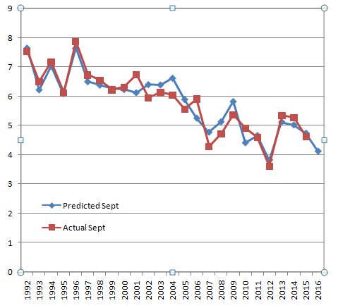
Rob Dekker, 5.4 (Std. Dev.=0.34), Statistical. My projection is based on an estimate of how much heat the Northern Hemisphere absorbs during spring and early summer. I use three variables (land snow cover, ice concentration, ice area) that are available in June, in a formula which shows particularly strong correlation with Sept sea ice extent. Regressed over the1992 - 2015 period, the formula projects 4.1 M km^2 for September 2016, with a standard deviation of only 340 k km^2.
Past performance of this June forecast method for September ice extent over the past 24 years shown in a graph here. The interesting finding is that the June land snow cover signal is clearly present in the September ice extent numbers.
Zhan, Yizhe, 5.46 (±0.3), Statistical. We estimated the September sea ice extent in 2017 to be much larger than last year. Compared to June 2016, MISR (firstlook product) indicates a significant increase in RSR over both the Canadian Arctic Archipelago and Svalbard, which consistent with the sea ice concentration anomaly. The area-weighted Pan-Arctic mean June RSR 2017 is much larger than that in 2016 and only slightly smaller than 2014.
Individual Outlook PDFs
| Attachment | Size |
|---|---|
| AWI Consortium (Kauker et al.)89.43 KB | 89.43 KB |
| Barthélemy et al.92.29 KB | 92.29 KB |
| Bosse80.6 KB | 80.6 KB |
| Brettschneider et al.83.03 KB | 83.03 KB |
| Cawley76.21 KB | 76.21 KB |
| CIS (Tivy et al.)546.42 KB | 546.42 KB |
| CNRM (Chevallier et al.)90.05 KB | 90.05 KB |
| CNRM System 693.08 KB | 93.08 KB |
| CPOM83.07 KB | 83.07 KB |
| Dekker93.9 KB | 93.9 KB |
| FIO-ESM (Qiao et al.)83.51 KB | 83.51 KB |
| GFDL/NOAA (Bushuk et al.)96.21 KB | 96.21 KB |
| Ionita and Grosfeld82.31 KB | 82.31 KB |
| John78.6 KB | 78.6 KB |
| Kondrashov83.41 KB | 83.41 KB |
| Lamont (Yuan et al.)100.76 KB | 100.76 KB |
| McGill (Tremplay et al.)87.47 KB | 87.47 KB |
| Meier, NASA Goddard89.99 KB | 89.99 KB |
| Met Office96.98 KB | 96.98 KB |
| Modified_CanSIPS107.37 KB | 107.37 KB |
| Morison80.16 KB | 80.16 KB |
| MPAS-CESM (Cavallo et al.)87.09 KB | 87.09 KB |
| NASA GMAO87.77 KB | 87.77 KB |
| NCAR/CU (Kay et al.)79.52 KB | 79.52 KB |
| NESM92.04 KB | 92.04 KB |
| NMEFC (Li and Li)81.17 KB | 81.17 KB |
| Petty81.6 KB | 81.6 KB |
| RASM (Kamal et al.)88.09 KB | 88.09 KB |
| Sanwa School77.4 KB | 77.4 KB |
| Slater/Barrett NSIDC84.16 KB | 84.16 KB |
| Nico Sun76.54 KB | 76.54 KB |
| UTokyo (Kimura et al.)86.1 KB | 86.1 KB |
| Wang et al.76.83 KB | 76.83 KB |
| Wu and Grumbine83.33 KB | 83.33 KB |
| Zhan80.7 KB | 80.7 KB |
| Zhang and Schweiger238.75 KB | 238.75 KB |
| Pan-Antarctic Reid et al.78.22 KB | 78.22 KB |
| Pan-Antarctic Antarctic Gateway Partnership (Davies)74.12 KB | 74.12 KB |
| Regional Druckenmiller and Eicken3.17 MB | 3.17 MB |
| Regional Gudmandsen217.25 KB | 217.25 KB |
| Informal AWI Cryosat530.9 KB | 530.9 KB |
| Informal Viddal52.01 KB | 52.01 KB |
