
Full Outlook Report
Summary
Thank you to the groups that contributed to the 2015 August Report. We have 38 (including one regional only) contributions, which again sets a new record for the total number of submissions.
The median August Outlook for September 2015 Arctic sea ice extent is 4.8 million square kilometers (km2), 200,000 km2 lower than the June and July medians. The quartile range is 4.2 to 5.2 million km2 (see Figure 1 in the Overview section, below). Contributions are based on a range of methods: statistical, dynamical models, estimates based on trends, and subjective information. The overall range (excluding an extreme outlier) is 2.7 to 5.6 million km2. The low end of the range dropped substantially from July (3.3 million km2), due to one new contribution, while the high end changed only slightly from July (5.7 million km2).
The median's decrease from the June and July values reflects rather rapid ice loss during July. The drop is mostly due to lower statistical and mixed statistical/heuristic contributions (Figure 2), because these methods are generally at least partially based on extrapolation from current/previous conditions whereas modeling contributions are generally not.
The August Outlook was developed by lead author Walt Meier (NASA Goddard Space Flight Center) with contributions from the rest of the SIPN leadership team. This month's report includes a compilation of ship-based observations from the Geographic Information Network of Alaska IceWatch program, a discussion of the August modeling contributions and how they compare to June and July, a look at the predictions in specific regions, and a discussion of current ice and weather conditions.
Overview
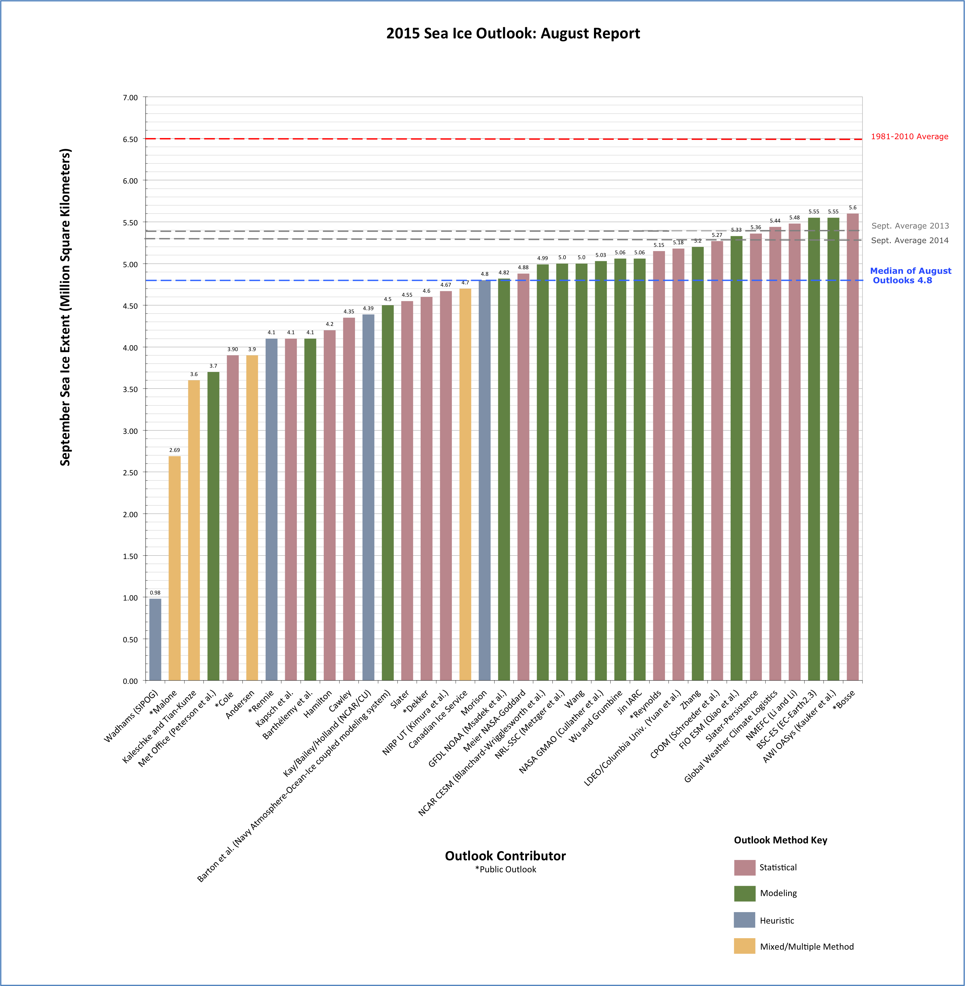
The Arctic Sea Ice Outlook contributions this August are based on a range of methods: statistical, dynamical models, estimates based on trends, and subjective information. We again have a record number of contributions (38, one of which is regional only) and value the diversity they include. The median August Outlook for September 2015 Arctic sea ice extent is 4.8 million square kilometers km2 (Figure 1). The quartile range is 4.2 to 5.2 million km2 and the overall range (excluding an extreme outlier) is 2.7 to 5.6 million km2. The low end of the range dropped substantially from July (3.3 million km2), due to one new contribution, while the high end changed only slightly from July (5.7 million km2).
Eighteen contributions updated their forecast for August, and there were two new contributions, resulting in slight changes in distribution. The biggest shift in median estimates came from the statistical methods, which dropped from slightly above 5.0 million km2 to about 4.8 million km2. The mixed statistical/heuristic methods also dropped noticeably. This makes sense because both approaches are generally based on previous data and current conditions at the time of the forecast. Thus, because July showed a substantially faster-than-normal rate of ice loss, methods that used this information to revise their estimates showed a reduced forecast for the September mean extent. Interestingly, the quartile range of the statistical methods is substantially lower, due mostly to a narrowing of the range on the low end. Thus, even with the rapid July ice loss rates, the lowest statistical estimates were revised upwards.
The median of the model contributions dropped only slightly from July and has been quite consistent throughout all three Outlooks. This in part reflects the fact that not all modeling contributions updated their forecasts with current conditions. Nevertheless, 10 modeling contributions did provide updated forecasts, with four showing an increase and the rest a decrease.
 for September 2015 sea ice extent.")
Download a high-resolution version of Figure 1.

Changes in Contributions from June and July Reports
Eighteen contributions provided an updated estimate for the August report. These are tabulated in Table 1 below. Interestingly, eight of those contributions showed an increase in the forecasted mean September extent despite the fast pace of ice loss seen in July and that by the end of July, the extent was tracking below that observed in 2013 and 2014.
| Name | Method | August Outlook | Change from July | Change from June |
|---|---|---|---|---|
| Met Office (Peterson et al.) | Modeling | 3.7 | -0.7 | |
| Barthélemy et al. | Modeling | 4.1 | -0.1 | -0.4 |
| Wu and Grumbine | Modeling | 5.06 | 0.06 | 0.46 |
| Morison | Heuristic | 4.8 | -0.7 | 0 |
| Yuan et al. (LDEO/Columbia) | Modeling | 5.18 | 0.1 | 0.19 |
| Barton et al. (Navy) | Modeling | 4.5 | -0.57 | |
| Msadek et al. (NOAA-GFDL) | Modeling | 4.82 | -0.03 | -0.35 |
| Zhang | Modeling | 5.2 | 0.1 | 0 |
| Metzger et al. (NRL) | Modeling | 5 | -0.3 | -0.2 |
| Slater-Persistence | Statistical | 5.36 | 0.2 | 0.14 |
| Global Weather & Climate | Statistical | 5.44 | -0.11 | -0.1 |
| Kauker et al. (AWI/OASys) | Modeling | 5.55 | -0.03 | -0.12 |
| Wang | Modeling | 5 | -0.07 | |
| Cole | Statistical | 3.9 | 0.64 | |
| Rennie | Statistical | 4.1 | 0.3 | |
| Slater | Statistical | 4.55 | 0.02 | |
| Meier | Statistical | 4.88 | -0.21 | |
| Qiao et al. (FIO-ESM) | Modeling | 5.33 | 0.03 | |
| Malone | Mixed | 2.69 | New in August | |
| BSC-ES (EC-Earth2.3) | Modeling | 5.55 | New in August |
Comment on Dynamical Model Predictions
Provided by François Massonnet, Université catholique de Louvain, Belgium, & Catalan Institute of Climate Sciences, Spain
We received 14 outlooks from dynamical modeling groups (see Figure 3) for the August round of submissions. Ten of them submitted updated values as compared to July, three resubmitted their July outlook, and we welcomed one new contributor (BSC-ES). Nine contributions stemmed from fully-coupled dynamical models, and five from ocean-sea ice models forced by atmospheric reanalyses or atmospheric model output.
 and green (ocean-sea ice). Values for June and July are shown in lighter colors. The dots are the outlook estimates themselves and the intervals are the uncertainty ranges provided by the groups. Definitions of uncertainty were left to the discretion of the groups themselves, and should therefore be compared with caution. The middle dashed horizontal line is the median of the August outlooks from dynamical modeling groups. The lower and upper dashed horizontal lines show, respectively, the lowest and highest bounds for all August modeling contributions. Figure courtesy of François Massonnet.")
We compared various data (see Table 2, below) from the modeling contributions over the three-month span of the 2015 outlook. Compared to the 2014 Sea Ice Outlook reports, the median predicted extent remained relatively stable for June, July, and August this year.
| Data for 2015 Modeling Contributions | June | July | August |
|---|---|---|---|
| Number of submissions (new/updated) | 11 (11) | 12 (7) | 14 (11) |
| Median extent (mean) in million km2 | 5.1 (5.1) | 5.1 (5.0) | 5.0 (4.9) |
| Inter-model standard deviation in million km2 | 0.41 | 0.41 | 0.5 |
| Inter-model range in million km2 | 1.3 | 1.5 | 1.8 |
| Estimated mean standard deviation in million km2 | 0.45 | 0.49 | 0.43 |
The evolution of uncertainties is, however, more puzzling. In 2014, both inter-model spread and spread between members of individual members tended to shrink for later submissions. This suggested that dynamical models were more confident (individually and as a group) as more information was integrated in the prediction systems. This is not the case in 2015.
There are two possible explanations for why we don't benefit from more confident predictions in 2015. The first one is to recognize that the size of the sample is small (14) and that our statistics for both 2014 and 2015 are noisy. The conclusions obtained last year are supported by results from peer-reviewed literature (e.g., Day et al., 2014), so we could suggest that results of 2015 are unexpected, statistically speaking. The second explanation would be that there are actually years that are truly more unpredictable than others, and 2015 would be one of them. Figure 3 shows that the spread of members of the same model can increase, in some models, from June to August (e.g., the NRL submission). What causes variance to increase (or at least not decrease) in some models has yet to be identified.
In summary, dynamical models predict a median September extent of 5.0 million km2 but with a large range in the estimates for the September minimum (3.7 to 5.55 km2). This large spread in the predictions reflects the current diversity in the formulation of physics and initial conditions in the various models used, but also inherent uncertainty of the climate system.
Day, J.J., S. Tietsche, E. Hawkins (2014) Pan-Arctic and Regional Sea Ice Predictability: Initialization Month Dependence. Journal of Climate, Vol 27, pp. 4371-4390, doi:10.1175/JCLI-D-13-00614.1.
Comment on Regional Predictions
We had one regional Outlook this month for the Nares Strait region (Gudmandsen). Dominant southerly winds throughout July and early August have prevented the drift of sea ice through Nares Strait into Baffin Bay even though the break-up of the ice barrier occurred in early July. The warm southerly winds also accelerated the melt of first-year ice in area. Continued melt and/or strong northerly winds are required for a change in conditions; drift of multi-year ice from the Lincoln Sea through Nares Strait is expected by the end of the month.
We also received 3 submissions of sea ice probability (SIP) for the August report, two of them from dynamical models (NRL-SSC/Metzger et al. and UK MetOffice/Peterson et al.) and one from a statistical model (Slater). These are shown in Figure 4.
, in the Slater, NRL-SSC/Metzger et al., and MetOffice/Peterson et al. forecasts. The MetOffice forecast is not bias corrected and has a slight negative overall bias.")
Compared to the earlier SIP submission in June, SIPs are notably lower in the Beaufort Sea, but higher in Laptev/Kara sectors.
According to the NRL-SSC/Metzger et al. contribution, compared to the July outlook an earlier ice-free date (IFD) is forecast in the East Siberian Sea (see Figure 5, below). However, this is also the region with the most uncertain forecast dates as shown by the high standard deviation (Figure 5, left-hand side).
. Right: Standard deviation of the IFD, with grey indicating a data void (i.e., no ice free days as the most likely outcome) of the projected GOFS 3.1 ensemble September mean for 2015. Images courtesy of NRL-SSC/Metzger et al.")
Current Conditions
In stark contrast to the relatively slow ice loss during June, July saw quite rapid ice loss (Figure 6), with rates averaging over 100,000 km2 per day through the month. The large losses in July brought the extent closer to 2012 end-July values. Relatively large daily ice losses have continued into early August, though they are less than the extreme losses in early August 2012 that occurred in the wake of a strong cyclone that moved through the area and broke up the ice in the Chukchi Sea.
, 2012 (dashed green), and the 1981-2010 average (black) and standard deviation (gray). From the NSIDC Arctic Sea Ice News and Analysis.")
Interestingly this year, while July ice loss rates were rapid in the central Arctic, melt out of the seasonal ice in Hudson and Baffin bays was slow with the ice cover persisting longer than in recent years. In the Arctic Ocean, the largest losses have been in the Beaufort and Chukchi Seas where large open water areas opened up within the ice pack. Sea surface temperatures were warm in coast areas, but near-freezing in the open water areas within the ice pack, which is expected given the recent ice melt in that region (Figure 7).
 UpTempO buoys. Figure courtesy of the University of Washington Polar Science Center.")
The large losses in July are likely related to strong high pressure over the North Pole (Figure 8), resulting in relatively clear skies and divergence within the ice pack. The high sea level pressures in July are the opposite of the long-term climatology for the summer Arctic. However, the occasional presence of these higher pressures has been a feature of the last decade and support sea ice loss. In August, the center of the high pressure region shifted to over the Kara Sea, while low surface pressure emerged over the Beaufort Sea.

Air temperatures (at the 925 mb level) were much higher than normal over the central Arctic (Figure 9), 1 to 2 ˚C above average over much of the region, with small areas in the East Siberian Sea and just north of Greenland over 4 ˚C above normal. The anomalously warm region shifted in August with warmest air centered over Svalbard, extending to the North Pole. It was also quite warm in parts of the Canadian Archipelago. The only region cooler than normal was in the Beaufort Sea where temperatures were 1 to 2 ˚C cooler than the 1981-2010 average. These cooler conditions continued into mid-August, with substantial freezing of melt ponds reported from a USCG flight over the region in early August.

Currently, the ice extent is tracking below that observed in 2010, 2013 and 2014, making the daily extent the 4th lowest in the satellite data record. The Northern Sea Route is open while significant parts of the Northwest Passage remain clogged with ice. Some channels in the Northwest Passage are opening, particularly along the famed Amundsen Route, so it may yet open before the melt season ends. Since there is still likely another month of ice loss to go, there is high probability that the September mean extent will drop below 5 million km2. As of August 18th, the extent is at 5.66 million km2.
Ship Observations of Conditions from IceWatch
Ice Watch has received observational reports of ice conditions from several cruises, some of which are summarized below and in Table 3. Data and maps of the cruise data can be accessed at: http://icewatch.gina.alaska.edu. We are expecting reports from the Polarstern and more Lance/N-ICE supply cruises at a later date. August through October we will be receiving further observations from the R/V Healy GEOTRACES campaign and the CCGS Louis S. St. Laurent JOIS cruise.
K/V Svalbard
Observations were recorded during supply cruises to support the R/V Lance during the N-ICE campaign, a drifting station set north of Svalbard. Only observations from the first cruise have been provided to date, however later cruise data will be provided once observers have processed it and completed quality control.
R/V Sikuliaq
Alice Orlich provided observations from the Sikuliaq ice trials cruise in the Bering Sea. Please note, only preliminary data has been provided and the full data set is not available online.
50 Let Pobedy
This is the first year we have received observations recorded by tourists. Tour leaders have been trained in observations and are in contact with sea ice experts, however it should be noted this is their first experience recording these observations. Two cruises, out of four planned for this summer, have reported conditions along a repeating cruise track.
- Roughly equal areas of first year and multi-year ice were encountered, within the central Arctic pack between Franz Josef Land and the North Pole.
- Preliminary reports from leg 3 are rotten ice, extensive towards ice edge at Franz Josef Land, and melt ponds freezing over.
| Ship | Dates | Region | Mean z (cm) | Median z (cm) | Type | Mean z (cm) | Median z (cm) | Type |
|---|---|---|---|---|---|---|---|---|
| R/V Sikuliaq | 2015/3/26-2015/4/2 | Bering Sea | 30 | 25 | FY | |||
| K/V Svalbard | 2015/01/12-2015/01/17 | N. Svalbard | 90 | 90 | FY | |||
| 50 Let Pobedy | 2015/07/13-2015/07/26 | To North Pole | 163 | 160 | MY | 86 | 80 | FY |
| 50 Let Pobedy | 2015/07/23-2015/07/26 | To North Pole | 172 | 160 | MY | 91 | 100 | FY |
Key Statements/Executive Summaries From Individual Outlooks
The Outlooks are listed below in order of lowest to highest predicted September extent. Extent and uncertainty (in parentheses) values are provided below in units of millions of km2 unless noted otherwise. The individual outlooks can be downloaded as PDFs at the bottom of this webpage.
Wadhams (Sea Ice and Polar Oceanography Group), 0.98, Heuristic (same as June)
We use entirely statistical extrapolation methods based on measured values of sea ice extent (from satellites) and sea ice thickness (from submarine voyages). [Editor's Note: Upon review by the SIPN team, this outlook has been listed as heuristic in the Sea Ice Outlook report.]
Malone, 2.69, Heuristic/Statistical
Using a mixed statistical-heuristic method, I am predicting final sea ice extent of approximately 2.48 million km2 by approximately 09/18/2015 (September 17th, 2015) with a September monthly average of 2.69 million km2. This estimate was developed initially using a few heuristics. Based on 2013-2014 observations, I believe solar decline in the face of increasing greenhouse forcing is likely to offset one another. 2012 had an El Nino, and once I started to see some signs of a developing system, I used the 2012 curve to account for the additional heat and adjusted the 2012 numbers to start at the end of the final curve from 2014. This model held within standard 95% confidence intervals until about July 5th, when cloud cover significantly reduced solar forcing. Once the heavy cloud systems passed, I realigned the remaining 2012 data from July 5th and the model has held ever since.
Kaleschke and Tian-Kunze, 3.6 (± 0.7), Heuristic/Statistical (same as June)
Based on February/March SMOS sea ice thickness and September SSMI sea ice concentration we provide a heuristic/statistical guesstimate for the 2015 September sea ice extent: 3.6 (±0.7) million km2. We use the product of the long-term average September SSMI ASI sea ice concentration and the February/March SMOS sea ice thickness as a predictor for the September extent. A threshold h applied on the (thickness Feb = Mar concentration Sept) field yields the predicted September extent after the regression with the past four years of sea ice extent observations. A threshold of h = 1.05m resulted in a correlation of R2 = 0.96 for the four years 2011, 2012, 2013 and 2014. The method applied to February/March 2015 predicts 2.8 million km2 for September. Our guesstimate is the average of the SMOS based prediction and the long term trend (4.3 million km2) with the difference of both as uncertainty.
Met Office (Peterson et al.), 3.7 (± 0.7), Modeling
Using the Met Office GloSea5 seasonal forecast systems we have generated a model based mean September sea ice extent outlook of 3.7 (± 0.7) million km2. This has been generated using startdates between 22 July and 10 August to generate an ensemble of 41 members (and 1 failed member). Note: Given current capabilities for seasonal forecasting of sea ice, we consider this still an experimental forecast.
Andersen, 3.9, Statistical/Heuristic (same as June)
I continue to use the same method based on the maximum area in spring at the relatively stable reduction fraction we have seen the last 8 years. Based on the data produced by NERSC my prognosis for minimum value of the area for 2015 is 3.9 million km2. That implies just slightly more than the then record low of 2007. For more description on the method used by Andersen, please see the Andersen PDF from the 2012 SIO.
Cole, 3.9 (±0.17), Statistical
The purpose of this contribution is to make use of the extent of high-concentration ice on August 5 as a predictor of the September extent. The region of ice concentration >60% on August 5 from MyOcean (TOPAZ4 model) was used as a predictor variable, and a linear regression was performed of September NSIDC extent vs. >60% concentration area on August 5. The years used to determine the slope and intercept of the regression line are 2012-2014. Area was determined using pixel counting in MATLAB, beginning from downloadable PNG file.
Kapsch et al., 4.1 (±0.5), Statistical (same as June)
For the prediction of the September sea-ice extent we use a simple linear regression model that is only based on the atmospheric water vapor in spring (April/May). Thereby we assume that the spring atmospheric conditions, more precisely the greenhouse effect associated with the water vapor in the atmospheric column, are important for the seasonal prediction of the September sea-ice extent.
Rennie, 4.1 (±0.2), Heuristic
This estimate is primarily based on the distribution of the April PIOMAS sea ice volume estimate taking into account the extent of ice represented by various thicknesses. There appears to be a fairly consistent rate of loss measured by original thickness through until the end of July. Predicting the final figure for mid- September is much more problematic and is heavily influenced by June to Sept weather. The methodology is similar to the starting point for my estimate last year which proved to be extremely low. This years' estimate is modified to accommodate additional factors and takes into account last years' experience and factors that may have resulted in that figure being too low. These include:
- The importance of a sequence of warm years to prepare the ice for a significant melt season.
- The summer temperatures from May-Sept.
- The April extent that was covered by ice estimated at between 1.5 and 2.5 m thick which, according to this methodology, would melt out at the end of the season.
- The observation that over the past 15 years there appears to be a developing correlation between the duration when the extent is within 200 km2) of the winter maximum and the depth of the decline.
Barthélemy et al., 4.1 (3.3-4.6), Modeling
Our estimate is based on results from ensemble runs with the global ocean-sea ice coupled model NEMO-LIM3. Each member is initialized from a reference run on July 31, 2015, then forced with the NCEP/NCAR atmospheric reanalysis from one year between 2005 to 2014. Our estimate is the ensemble median, and the given range corresponds to the lowest and highest extents in the ensemble.
Hamilton, 4.2 (±1.0), Statistical (Same as July)
A Gompertz (asymmetric S curve) model estimated by iterative least squares, looking one year ahead, suggests a mean September 2015 ice extent of 4.2 million km2. Past variations suggest a 95% confidence interval for this prediction ranging from 3.2 to 5.2 million km2 (+/- 1.0).
Cawley, 4.35 (±1.16), Statistical (Same as July)
This is a purely statistical method (related to Krigging) to estimate the long term trend from previous observations of September Arctic sea ice extent. As this uses only September observations, the prediction is not altered by observations made during the Summer of 2015.
Kay et al. (NCAR), 4.39 (Std dev = 0.45), Heuristic (Same as June)
An informal pool of 30 climate scientists in early June 2015 estimates that the September 2015 ice extent will be 4.39 million km 2 (std dev. 0.45, min. 3.25, max. 5.15). Since its inception 8 years ago, the NCAR/CU sea ice pool has easily rivaled much more sophisticated efforts based on statistical methods and physical models to predict the September monthly mean Arctic sea ice extent (e.g. see appendix of Stroeve et al. 2014 in GRL doi:10.1002/2014GL059388 ; Witness the Arctic article by Hamilton et al. 2014. We think our informal pool provides a useful benchmark and reality check for Sea Ice Prediction efforts based on more sophisticated physical models and statistical techniques.
Barton et al. (Navy Atmosphere-Ocean-Ice coupled modeling system), 4.5 (±0.3), Modeling
The projected Arctic minimum sea ice extent from the Navy’s global coupled atmosphere-ocean-ice modeling system is 4.5 million km 2. This projection is the average of an eight member ensemble. The range of the ensemble is 4.2 to 4.8 million km 2. Note that our ensemble
range does not represent a full measure of uncertainty, and the system is currently in a development stage.
Slater, 4.55 (±0.35), Statistical
I have extended my model prediction out to a lead time of 53 days. The method is effectively the same as my “standard” 50 day forecast. The method has real skill (as measured by Schröder et al. [2014]) at 53 days over the period 1995-2013. I believe this forecast has equal or greater skill at this lead time than the Schröder et al. method.
Dekker, 4.6 (Std dev = 0.37), Statistical (Same as July)
The basic concept behind my method pertains to estimating albedo-based Arctic amplification during the melting season. I use the "whiteness" of the Arctic in June as a predictor for how much ice will melt out between June and September. Specifically, I use a formula based on physics of energy absorption, using snow cover, and June ice extent/area numbers. The interesting result is that not only the standard deviation (at 370 k km2) is significantly better than the 500 k km2 or so that would be achieved for a simple linear trend, but also this method explains a large part of the increase in September ice extent during the 2013 and 2014 season w.r.t. 2012 and other years. For 2015, this method predicts that there will NOT be a repeat of the 2013 and 2014 5 million+ extent, but instead ice extent in September will be 4.6 million km2 (±370 k km2).
NIPR/UT (Kimura et al.), 4.67, Statistical (Same as July)
The monthly mean ice extent in September will be about 4.67 million km2. Our estimate is based on a statistical way using data from satellite microwave sensor. We used the ice thickness in December, ice movement from December to April, and ice concentration in June. Predicted ice concentration map from July to September is available in our website: http://www.1.k.u-tokyo.ac.jp/YKWP/2015arctic2_e.html.
Canadian Ice Service, 4.7 (±0.2), Heuristic/Statistical (same as June)
The 2015 forecast was derived by considering a combination of methods: 1) a qualitative heuristic method based on observed end-of-winter Arctic ice thickness extents, as well as winter Surface Air Temperature, Sea Level Pressure and vector wind anomaly patterns and trends; 2) a simple statistical method, Optimal Filtering Based Model (OFBM), that uses an optimal linear data filter to extrapolate the September sea ice extent timeseries into the future and 3) a Multiple Linear Regression (MLR) prediction system that tests ocean, atmosphere and sea ice predictors. The average forecast value of the three methods combined is 4.7 million km2.
Morison, 4.8 (±0.5), Heuristic (Same as June)
My estimate of 4.8 million km2 is based on prior years’ ice and Arctic Oscillation index plus in situ observations of ice in April and June.
GFDL NOAA (Msadek et al.), 4.82 (4.33-5.23), Modeling
Our prediction for the September-averaged Arctic sea ice extent is 4.82 million square kilometers, with an uncertainty range going between 4.33 and 5.23 million km2 Our estimate is based on the GFDL CM2.1 ensemble forecast system in which both the ocean and atmosphere are initialized on August 1 using a coupled data assimilation system. Our prediction is the bias-corrected ensemble mean, and the given range corresponds to the lowest and highest extents in the 10- member ensemble. Our model predicts that September 2015 Arctic sea ice extent will be 2.14 million km 2 below the 1982 to 2011 observed average extent, but will not reach values as low as those observed in 2007 or 2012.
Meier (NASA Goddard), 4.88 (±0.43), Statistical
This method is a simple statistical method that uses previous years’ daily rates of extent change to project the 2015 daily extent through the end of September. The monthly average is then calculated from the September daily extents. This year, the last ten years (2005 – 2014) are used for the projection because these years are more representative of recent conditions than using all years in the 35-year time series. This method yields a September 2015 extent of 4.88 (±0.43) million km2.
Blanchard-Wrigglesworth et al. (NCAR CESM), 4.99 (±0.47), Modeling (Same as July)
Our July Outlook for September 2015 is 4.99 million km2. We have used the NCAR CESM global fully coupled model to make this prediction. Our uncertainty is 0.47 million km2.
Wang, 5.0 (±0.27), Modeling
A projected September Arctic sea ice extent of 5.0 million km2 is based on a NCEP ensemble mean CFSv2 forecast initialized from the NCEP Climate Forecast System Reanalysis (CFSR) that assimilates observed sea ice concentrations and other atmospheric and oceanic observations. Raw forecast output is bias corrected based on the systematic of the forecast for recent years. The uncertainty is estimated as the root mean square (rms) error of the ensemble mean based on CFSv2 hindcasts (1982-2010) and forecasts (2011-2014). Estimated error is ±0.27 million km2.
Metzger et al. (NRL Stennis Space Center), 5.0 (3.4-6.0), Modeling
The Global Ocean Forecast System (GOFS) 3.1 was run in forecast mode without data assimilation, initialized with July 1, 2015 ice/ocean analyses, for ten simulations using National Centers for Environmental Prediction (NCEP) Climate Forecast System Reanalysis (CFSR) atmospheric forcing fields from 2005-2014. The mean ice extent in September, averaged across all ensemble members is our projected ice extent. The GOFS 3.1 outlook for the 2015 September minimum ice extent is 5.0 million km2 with a range of 3.4 – 6.0M km2.
NASA GMAO (Cullather et al.), 5.03 (±0.41), Modeling (Same as June)
The GMAO seasonal forecasting system predicts a September average Arctic ice extent of 5.03 (±0.41) million km2, about 4.7 percent less than the 2014 value. The forecast suggests reductions in ice extent along the Eurasian coast, but cooler near-surface air temperatures over the Canadian Archipelago. A positive summertime sea level pressure anomaly over the central Arctic Basin is featured. A significant aspect of the forecast is an exuberant prediction for strengthening of the current El Niño/Southern Oscillation (ENSO) warm phase and its accompanying interaction with the Pacific-North American mode at higher latitudes. This aspect and the proximity of the ENSO spring predictability barrier to the forecast initial time implies some additional uncertainty in this year's sea ice prediction.
Jin (IARC), 5.06, Modeling (same as June)
A coupled ice-ocean model forecast of the September sea ice extent minimum.
Wu and Grumbine, 5.06 (±0.58), Modeling
The projected Arctic minimum sea ice extent from the NCEP CFSv2 model with revised CFSv2 May-June-July ICs using 92-member ensemble forecast is 5.06 million km2 with a SD of 0.58 million km2. The Minimum and maximum values for the Arctic sea ice extent from the 92-member ensemble prediction are 3.67 and 6.42 million km2, respectively.
Reynolds, 5.15 (±0.64), Statistical (same as June)
The long-term loss of extent in summer is largely driven by volume decline of ice in the Arctic Ocean mediated by the resulting increase in open water formation efficiency. Based on this hypothesis the PIOMAS April average volume is calculated from PIOMAS gridded data and the relationship between April volume and September extent is used as a predictor. The resulting prediction is 5.15 million km2 +/- 0.64 million km2.
Yuan et al. (LDEO Columbia University), 5.18 (±0.38), Statistical
The prediction is made by statistical models that are capable to predict Arctic sea ice concentrations at grid points 2-month in advance with reasonable skill. The models employ 34 years of monthly time series of sea ice, SST and atmospheric variables. The pan Arctic SIE is calculated from predicted ice concentration and projected to be 5.18 million km2 in September 2015. That is lower than the observed extents in 2013 and 2014, but still above the historical low in 2012. The ice concentration is significantly below the 34-year climatology in the Beaufort Sea, Chukchi Sea, East Siberian Sea, Laptev Sea, Kara Sea and Barents Sea.
Zhang, 5.2 (±0.6), Modeling
Driven by NCEP/NCAR reanalysis data, PIOMAS is used to predict the total September Arctic sea ice extent as well as ice thickness field and ice edge location, starting on August 1. The predicted ice extent is 5.2 ±0.6 million km2.
CPOM (Schroeder et al.), 5.27 (±0.44), Statistical (Same as July)
We predict the September ice extent 2015 to be very close to 2013 and 2014, but considerably larger than in 2012. Although the air temperature was generally higher in June 2015 than in 2014, the melt-pond area in May and June is very similar to 2014 and below the 1979 to 2015 trend line. This is mainly due to a lower fraction of thin-ice in our model simulation in comparison to previous years.
Qiao et al. (FIO-ESM), 5.33 (±0.53), Modeling
Our prediction is based on FIO-ESM with data assimilation. The prediction is 5.33 (±0.53) million km2. 5.33 and 0.53 million km2 is the average and one standard deviation of 10 ensemble members, respectively.
Slater (Persistence), 5.36, Statistical
Three different types of persistence forecasting at 53-day or 2 month lead time. At this shorter lead time, the methods do contain skill (as measured by Schroder et al., [2014]).
Global Weather Climate Logistics, 5.44, Statistical
The Global Weather and Climate Logistic’s prediction is based on two statistical models that incorporate between 10 and 20 surface, atmospheric and oceanic variables. We are revising our August forecast down from our June prediction of 5.55 million km2 to 5.44 million km2 .
Li and Li (NMEFC), 5.48 (4.97-5.98), Statistical (Same as June)
We predict a September monthly average Arctic sea ice extent of 5.48 (4.97-5.98) million km2 using a statistical method. This is the same result as our June and July reports. Our sea ice prediction data sources come from the National Snow and Ice Data Center.
Kauker et al. (AWI/OASys), 5.55 (±0.38), Modeling
We estimate a monthly mean September sea-ice extent of 5.55 (±0.38) million km2 (without assimilation of sea-ice/ocean observations). The method is a sea ice-ocean model ensemble run (without and with assimilation of sea-ice/ocean observations); the coupled ice-ocean model NAOSIM has been forced with atmospheric surface data from January 1948 to 7 July 2015.
BSC-ES, EC (Earth2.3), 5.55 (Std dev = 0.43), Modeling
We produced this September 2015 forecast of Arctic sea ice conditions using a dynamical climate model (EC-Earth2.3) initialized on May 1st, 2015. This coupled general circulation model includes dynamic-thermodynamics model of sea ice (LIM2) with horizontal resolution of about 1 degree. We employ dynamical models for seasonal forecast because they have capability to resolve and predict details from pan-Arctic to local scales in non-stationary and physically consistent manner.
Bosse, 5.6 (±0.4), Statistical (Same as July)
As in the last year, I used two variables for a forecast of the September 2015 Sea Ice Extent: The Heat Content of the Arctic Ocean northward 65 deg. N form the summer of 2014 and the amount of sea ice volume ( PIOMAS) in the end of the winter (28.2.15).
Additional Regional Outlook
Gudmandsen, Nares Strait Region, Heuristic
A heuristic forecast for the timing of break-up in the Nares Strait region.
Please note that the SIO is not an operational forecast.
The original call for contributions for the August report is here.
Individual Outlook PDFs
 for September 2015 sea ice extent.")