
Summary
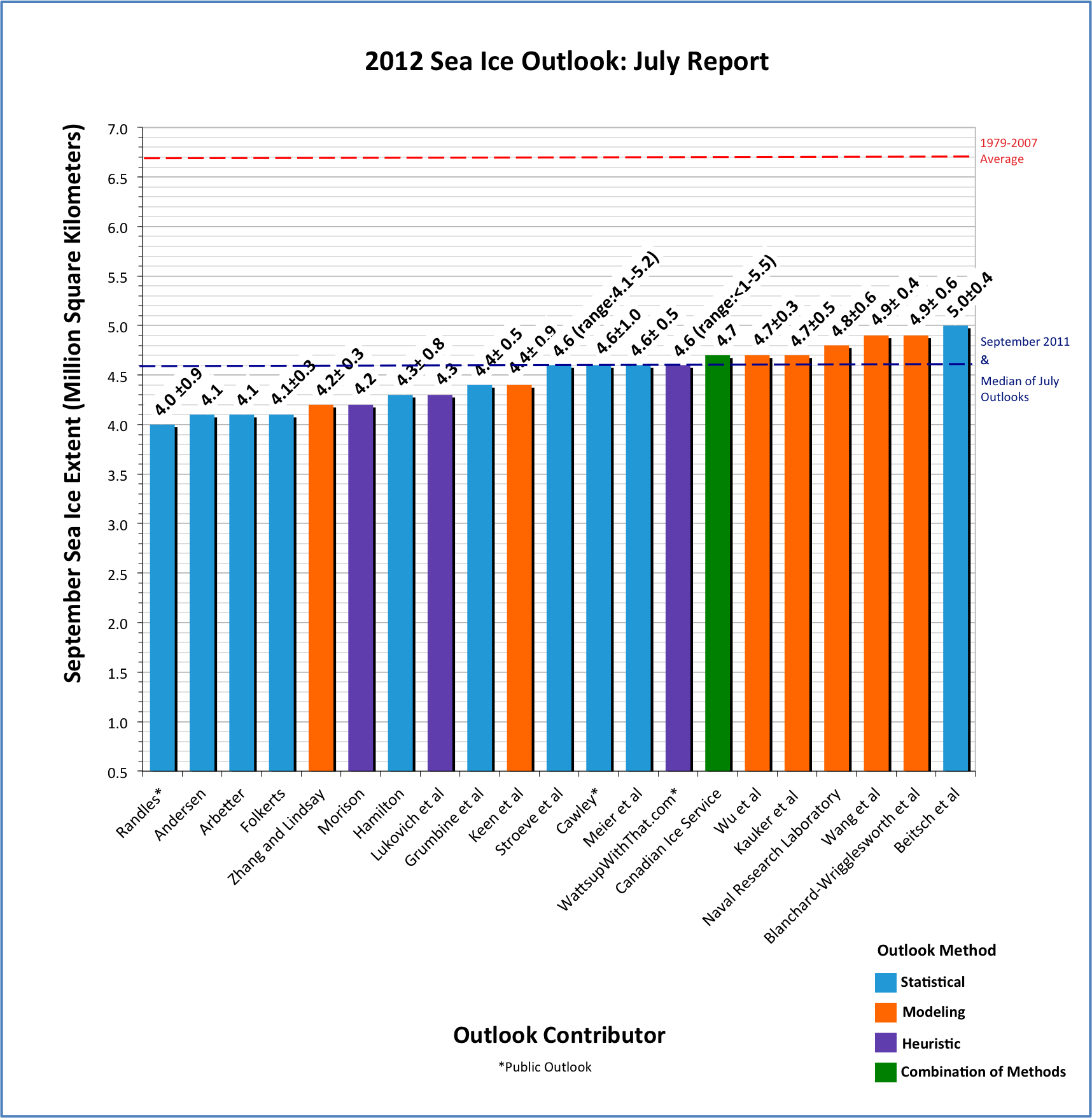
With 21 responses for the Pan-Arctic Outlook (plus 5 regional Outlook contributions), the July Sea Ice Outlook projects a September 2012 arctic sea extent median value of 4.6 million square kilometers (Figure 1). The consensus is for continued low values of September sea ice extent. Individual responses are based on a range of methods: statistical, numerical models, comparison with previous rates of sea ice loss, composites of several approaches, estimates based on various non-sea ice datasets and trends, and subjective information. Again, it is important to note for context that the estimates are well below the 1979–2007 September mean of 6.7 million square kilometers. The quartiles for July are 4.2 and 4.7 million square kilometers, a rather narrow range given that the uncertainty of individual estimates are on the order of 0.5 million square kilometers. This is also a narrower range than last year, which was 4.0 to 5.5. The July Outlook is generally similar to the June Outlook; the July median is higher by 0.2 million square kilometers than the June estimate, but the quartiles are similar.
Just after the June Outlook was completed (based on May data), arctic sea ice extent briefly set record daily rates of loss. In June we saw the second-most cumulative loss in the satellite record since 1979, behind the record minimum extent for June in 2010. We also saw cases of early melt in some regions. The culprit for the rapid sea ice loss in early June was again the presence of the Arctic Dipole (AD) pressure pattern, but the pattern shifted towards the end of the month and ice loss slowed.
 for September 2012 sea ice extent.")
The Pan-Arctic report was developed by Jim Overland, NOAA, Hajo Eicken, UAF, and Helen Wiggins, ARCUS. The Regional report was developed by Adrienne Tivy, National Research Council Canada, with assistance from Kristina Creek, ARCUS.
Pan-Arctic Full Outlook
OVERVIEW OF RESULTS
We appreciate the continuing contributions to the July Outlook (using June data). This critical number makes the activity worthwhile. We received 21 responses with a range of estimates from 4.0 to 5.0 million square kilometers for the September 2012 arctic mean sea ice extent (Figure 1). This generally mirrors the June 2012 Outlook and is a narrower range than last year, which went from 4.0 to 5.5. The median value for July is 4.6 million square kilometers and the quartile values are 4.2 and 4.7 million square kilometers, a rather narrow range given that the intrinsic uncertainty of the estimates are on the order of 0.5 million square kilometers. The July median is actually higher by 0.2 million square kilometers than the June estimate but the quartiles are similar. It should be recalled that we are comparing these Outlook values to the September average sea ice extent as provided by the National Snow and Ice Data Center (NSIDC). NSIDC is not the only data source for ice extent; their estimate is based on a long-term time series and we use their value as an operational definition. If other data sources for sea ice extent are used, the corresponding mean monthly ice extent values can be adjusted by an offset to roughly correspond to the NSIDC value.
JUNE 2012 ICE AND ATMOSPHERIC CONDITIONS
Just after the June Outlook was completed (based on May data), the sea ice extent loss rate became more than double the climatological rate (NSIDC, see Figure 2). Much was made of this major loss rate and low extent in the press and sea ice blogs. The major loss rate was particularly interesting given that we had considerable sea ice present in April (see last months discussion). However, in the second half of June 2012 the meteorological conditions changed and the rate of loss moderated. In June we saw the second-most cumulative loss in the satellite record since 1979, behind the minimum extent for June in 2010.
.")
The culprit for the rapid sea ice loss in early June was again the presence of the Arctic Dipole (AD) pressure pattern (Figure 3a). Normally (i.e., before 2007) low pressure and light winds prevail during summer in the Arctic. However, throughout the summer of 2007, the persistence of the Arctic Dipole Anomaly (AD) sea level pressure pattern, with high pressure on the North American side and low pressure on the Siberian side, contributed substantially to the record low ice extent in September 2007. In June 2010 and June 2011 the AD was only present in early summer, and in 2011 the pattern shifted toward the Siberian coast (Ogi and Wallace, GRL 2012). In early June 2012 we saw the classic AD pattern with implied winds across the central Arctic, east winds along the northern Alaskan coast, and sea ice advection out of the Fram Strait—all promoting sea ice loss. This AD pattern quickly shifted in the second half of June, however, and was replaced by a low sea level pressure center over the Pacific side of the Arctic Ocean (Figure 3b), opposing the transpolar sea ice drift.
 for early June 2012 showing an Arctic Dipole (AD) pattern over the central Arctic Ocean, but with stronger pressure gradients shifted toward the Siberian side.")
 for late June 2012 showing a more typical historical pattern with low SLP pattern over in the Pacific side of the Arctic Ocean.")
Sea ice extent for early July (Figure 4) shows not only anomalous open water areas in Baffin Bay, Hudson Bay, Kara Sea, and north of the Barents Sea, but also substantial open water areas within the central sea ice pack west of Banks Island and northeast of the New Siberian Islands. These open areas and that of the Kara Sea are consistent with thin sea ice and the AD weather pattern for early June. These early open water areas absorb the sun's energy, which help to further ice melt through the summer. Figure 5a shows that there was mostly open water at 71 N and 163 W in early July. The North Pole Environmental Observatory web camera also shows a shift to major melt pond formation in early July (Figure 5b). So for the September Outlook there are opposing factors; we have lost the AD pattern for now, but have regional examples of early melt. This is consistent with the July Outlook contributions that continue the course from the June Outlook, despite the early June sea ice losses.
.")
 marine mammal reconnaissance flight on 5 July 2012, in support of a project funded by the Bureau of Ocean Energy Management (BOEM).")

KEY STATEMENTS FROM INDIVIDUAL OUTLOOKS
Randles, 4.0, +/-0.9, Statistical If I were giving a heuristic estimate, I think I would make the estimate lower. However I think I will leave it at this naive statistical estimate as hopefully providing some sort of guide to how much more accurate estimates need to be as we get closer to the minimum in order to demonstrate skill over a naive statistical model like I am using.
Arbetter, 4.1, n/a, Statistical
Using conditions from week 22 of 2012 (ie June 1, 2012), a revised minimum Arctic sea ice extent is substantially lower than the first estimate of 4.32 million km2, using week 18 conditions (May 1, 2012), reflecting both lower than average sea ice extent used as initial conditions and a persistent downward trend in sea ice extent over the past decade (and longer). Based on these projections and previous model behavior, the output suggests 2012 will be at or below the previous record minimum September ice extent, set in 2007 and repeated in 2011.
Andersen, 4.1, Statistical
Same as last month.
Folkerts, 4.1, +/- 0.3, Statistical
It is reasonable to assume that past conditions of the ice, the Arctic climate, and wide-area climate indices should be correlated with future ice conditions. Because these relationships can be subtle and complex, statistical models combining multiple parameters are expected to be more effective than individual monthly data at making predictions.
Zhang and Lindsay, 4.2, +/-0.3, Model
These results are obtained from a numerical ensemble seasonal forecasting system. The forecasting system is based on a synthesis of a model, the NCEP/NCAR reanalysis data, and satellite observations of ice concentration and sea surface temperature. The model is the Pan-Arctic Ice-Ocean Modeling and Assimilation System (PIOMAS, Zhang and Rothrock, 2003). The ensemble consists of seven members each of which uses a unique set of NCEP/NCAR atmospheric forcing fields from recent years. In addition, the recently available IceBridge and helicopter-based electromagnetic (HEM) ice thickness quicklook data are assimilated into the initial 12-category sea ice thickness distribution fields.
Morison, 4.2, n/a, Heuristic
Same as last month.
Hamilton, 4.3, +/-0.8, Statistical
This is a naive model proposed at the start of the 2012 melt season. Most trend-line analyses of Arctic sea ice have used linear, quadratic, exponential or logistic models. The Gompertz curve appears preferable to these alternatives in several respects.
Lukovich et al., 4.3, n/a, Heuristic
Daily maps of surface winds, SLP, and nowcast ice drift data illustrate regional differences in atmospheric forcing of sea ice in 2011 and 2012. Noteworthy are maximum ice drift speeds through Fram Strait in early June, 2012 aligned with the interface between the SLP high and low regimes, observed to a lesser extent in late June of 2011. Increased variability in ice drift is also observed in 2012 compared to 2011. It is interesting to note that the anticyclonic circulation in the Beaufort Sea is preceded by a SLP high on June 14th, 2012, suggesting regional differences in ice drift response to surface winds, most likely due to regional differences in ice concentration and thickness.
Grumbine et al., 4.4, +/- 0.5, Statistical
Same as last month.
Keen et al. (UK Met Office-Hadley Centre), 4.4, +/-0.9, Model
This projection is based on results from the UK Met Office seasonal forecasting system GloSea4. Our projection is based on forecasts initialised between 12th March and 1st April 2012 inclusive (the choice of start dates is discussed in section 5 below), bias-corrected using hindcasts initialised on 9th and 17th March, and 1st April.
Stroeve et al. (NSIDC), 4.6, range 4.1-5.2, Statistical
Same as last month.
Cawley, 4.6, +/-1.0, Statistical
Same as last month.
Meier et al, 4.6, +/-0.5 Statistical
This statistical method uses previous years’ daily extent change rates from July 1 through September 30 to calculate projected daily extents starting from June 30. The September daily extents are averaged to calculate the monthly extent. Rates from recent years are more likely to occur because of the change in ice cover. Thus, the official projection is based on the rates for 2002-2011
**WatttsUpWithThat.com, 4.6, range
| Attachment | Size |
|---|---|
| Andersen93.47 KB | 93.47 KB |
| Arbetter351.78 KB | 351.78 KB |
| Beitsch et al.3.05 MB | 3.05 MB |
| Blanchard-Wrigglesworth et al.2.4 MB | 2.4 MB |
| Canadian Ice Service119.91 KB | 119.91 KB |
| Cawley49.33 KB | 49.33 KB |
| Folkerts369.97 KB | 369.97 KB |
| Grumbine et al.29.13 KB | 29.13 KB |
| Hamilton284.42 KB | 284.42 KB |
| Kauker et al.345.11 KB | 345.11 KB |
| Keen et al.352.05 KB | 352.05 KB |
| Lukovich et al.6.46 MB | 6.46 MB |
| Meier et al.214.04 KB | 214.04 KB |
| Morison34.1 KB | 34.1 KB |
| Naval Research Laboratory572.34 KB | 572.34 KB |
| Randles71.68 KB | 71.68 KB |
| Stroeve et al.576.72 KB | 576.72 KB |
| Wang et al.134.23 KB | 134.23 KB |
| WattsUpWithThat.com56.54 KB | 56.54 KB |
| Wu et al.38.82 KB | 38.82 KB |
| Zhang and Lindsay458.31 KB | 458.31 KB |
| Attachment | Size |
|---|---|
| Gerland et al.576.8 KB | 576.8 KB |
| Gudmandsen328.74 KB | 328.74 KB |
| Howell906.77 KB | 906.77 KB |
| Tivy476.63 KB | 476.63 KB |
| Zhang and Lindsay457.36 KB | 457.36 KB |
 for September 2012 sea ice extent.")