
EXECUTIVE SUMMARY
Thank you to the groups that contributed to the July 2014 Sea Ice Outlook; we received 28 pan-Arctic contributions and always appreciate the diversity of contributions.
The July Outlook report was developed by Walt Meier, NASA Goddard Space Flight Center, and the rest of the SIPN leadership team, with a section analyzing the model contributions by François Massonnet, Université Catholique de Louvain.
The median Outlook value for September 2014 sea ice extent is 4.8 million square kilometers with quartiles of 4.4 and 5.0 million square kilometers. Thus, the median value is slightly higher than the June value (4.7) and the distribution of Outlooks is slightly reduced relative to June. The overall range is now from 3.2 to 5.9 million square kilometers. These values compare to observed values of 4.3 million square kilometers in 2007, 4.6 million square kilometers in 2011, 3.6 million square kilometers in 2012, and 5.4 million square kilometers in 2013.
Sea ice declined at a pace more rapid than normal during June, particularly late in the month when extent decreased by over 100,000 square kilometers per day. The decline has since slowed somewhat.
The Sea Ice Outlook is a venue for discussion and networking and provides a transparent exercise in both scientific sea ice predictions as well as estimates from the public. The post-season activities will provide more of a scientific analysis of the methodologies, relative performance, etc.
This month's full report includes the comments on modeling outlooks and on regional predictions, a summary of current conditions, key statements from each Outlook, and links to view or download the full outlook contributions.
See the original call for contributions for the July report here.
Full Report
OVERVIEW
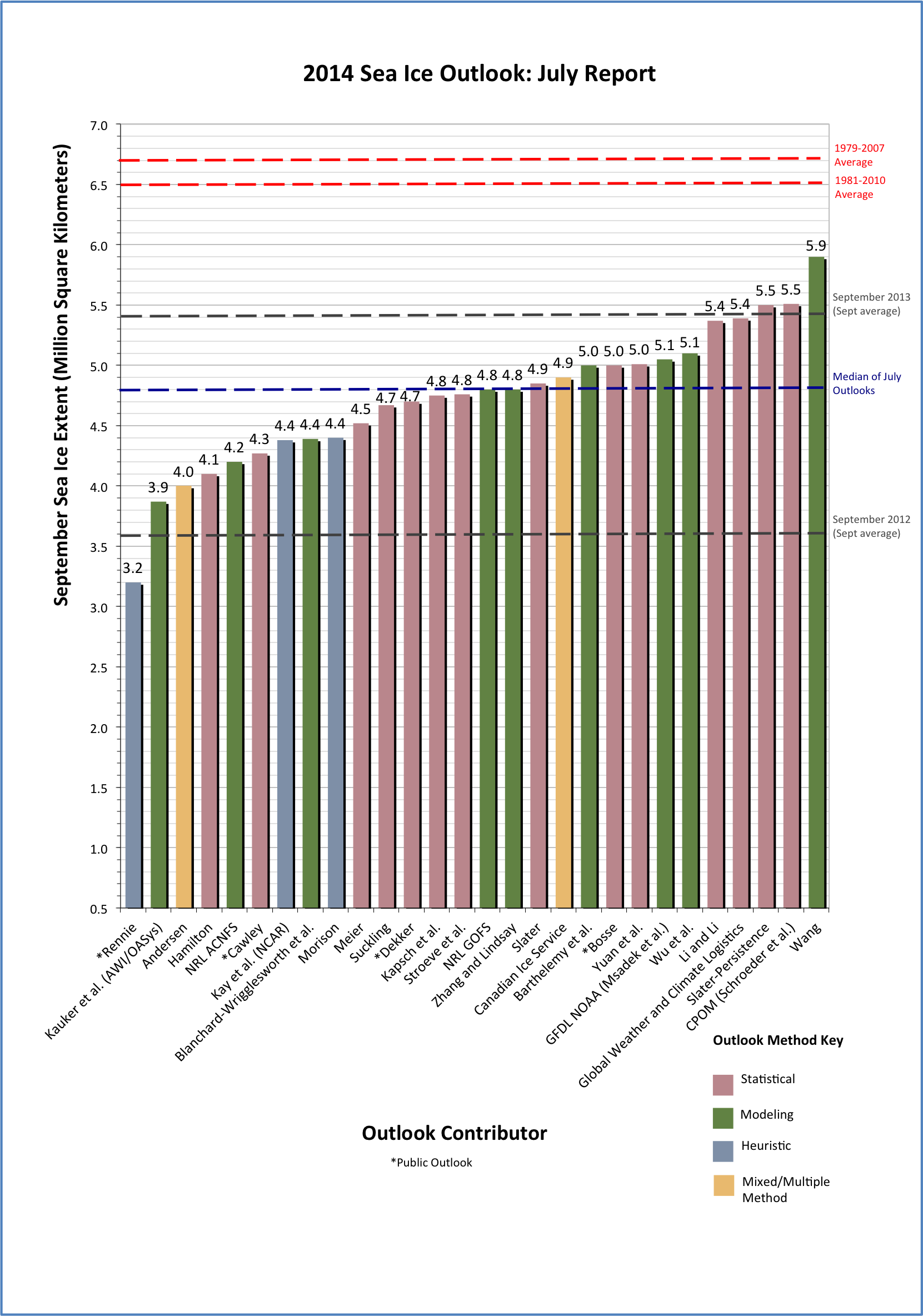
Thank you to the groups that contributed to the July 2014 season, we have received 28 pan-Arctic contributions matching the number for June. We appreciate the diversity of contributions. The median Outlook value for September 2014 sea ice extent is 4.8 million square kilometers with quartiles of 4.4 and 5.0 million square kilometers (See Figure 1). Thus the median value is slightly higher than the June value (4.7) and the distribution of Outlooks is slightly reduced relative to June. The overall range is now from 3.2 to 5.9 million square kilometers. These values compare to observed values of 4.3 million square kilometers in 2007, 4.6 million square kilometers in 2011, 3.6 million square kilometers in 2012, and 5.4 million square kilometers in 2013. Only three outlooks both in June and July are above the 2013 observed September extent (10% of all submissions). It is indeed an issue to separate the nominal downward trend in sea ice loss from year to year weather influences. A linear downward trend using the satellite period (1979-2013) would put 2014 at 4.7 million square kilometers. Based on previous years' SIO, weather in 2007 was a factor on the low side while weather in 2013 was a factor in the high side. More sea ice at the end of summer 2013 may be offset somewhat by a warm Arctic winter in 2013/2014. In terms of regional outlooks, we have only received a limited number of submissions, which nevertheless agree in showing a greater loss of sea ice off the coast of Alaska and Siberia relative to the European sector. We appreciate the addition of recent thickness data estimated from the European Space Agency (ESA) CryoSat-2 satellite, the NASA IceBridge airborne campaign, and Office of Naval Research (ONR) in situ buoys.
 for September 2014 sea ice extent (labels on the bar graph are rounded to the tenths for readability. Refer to the Individual Outlooks at the bottom of this report for the full details of individual submissions).")
Download High Resolution Version of Figure 1.
 and July (right) 2014 Outlook contributions as a series of box plots, broken down by general type of method. The box color depicts contribution method. A fifth box appeared in the June report separating out the modeling contributions that used both data assimilation and fully coupled modeling to arrive at their prediction. However, in July the number (n=3) of this type was too small to show as a distribution.")
COMMENT ON MODELING CONTRIBUTIONS
Provided by François Massonnet, Université Catholique de Louvain
There are nine contributions from modeling groups for the July outlook. The median predicted September sea ice extent amounts to 4.8 million km², slightly higher than the median prediction issued in June by the same groups. It is encouraging to note that the uncertainty around individual predictions is systematically lower or equal to that of June, suggesting that the predictions generally become more confident as new information is incorporated into the individual prediction systems. In a recent study, Day and colleagues (2014) pointed out the role of the initialization month on the predictability of September sea ice extent, in an idealized framework. They also showed that the ensemble spread is lower for later initialization dates, which is what we can see on Figure 3.

J. J. Day, S. Tietsche, E. Hawkins (2014) Pan-Arctic and Regional Sea Ice Predictability: Initialization Month Dependence. Journal of Climate, Vol 27, pp. 4371-4390, doi:10.1175/JCLI-D-13-00614.1
COMMENT ON REGIONAL PREDICTIONS
![Figure 4. Ensemble median prediction of September 2014 ice thickness and September 2014 ice edge location (black) from PIOMAS and the September 2013 observed ice edge (white) [Zhang and Lindsay]. Regions outlined in yellow show the Beaufort Sea and Barents Sea sea ice areas used in the statistical predictions[Global Weather and Climate Logistics].](/files/sio/21184/image007.png "Figure 4. Ensemble median prediction of September 2014 ice thickness and September 2014 ice edge location (black) from PIOMAS and the September 2013 observed ice edge (white) [Zhang and Lindsay]. Regions outlined in yellow show the Beaufort Sea and Barents Sea sea ice areas used in the statistical predictions[Global Weather and Climate Logistics].")
Three of the contributions provided regional predictions. The modeling submissions by Blanchard-Wrigglesworth et al. and Zhang and Lindsay both point to a greater sea ice loss off the coast of Alaska and Siberia compared to the European sector. This is consistent with the statistical forecast by Global Weather and Climate Logistics who predict a reduced September sea ice area in the Beaufort Sea and an increased sea ice area in the Barents Sea compared to 2013.
CURRENT CONDITIONS
Sea ice declined at a pace more rapid than normal during June, particularly late in the month when extent decreased by over 100,000 sq km per day. The decline has since slowed somewhat. The speed-up in the decline brought 2014 extent at the end of June to within 300,000 sq km of 2012 levels at the same time of year (Figure 5). This may portend a near-record September extent, if conditions were to evolve as in 2007 or 2010-2013, which were the only years with comparable ice extent in early July. However, there is still large uncertainty as to how the remainder of the Arctic melt season will progress in response to regional weather patterns and large-scale atmospheric circulation.
. From NSIDC Charctic Interactive Sea Ice Graph, http://nsidc.org/arcticseaicenews/charctic-interactive-sea-ice-graph")
By comparison, in 2012 areas of low concentration ice, indicating thinner and more broken floes, were already apparent within the ice cover (Figure 6). This year, most of the Arctic sea ice is still present at high concentrations, which indicates a more consolidated and possibly thicker, and thus potentially more resilient ice cover. At the same time, high concentrations may also indicate low melt-pond coverage, continuing a trend towards cooler surface conditions identified in the contribution by Schroeder et al. (CPOM) this month. Anecdotally, this is confirmed for the Chukchi Sea where pond coverage continued to be low well into June, as reported from shore-based and airborne observations.
 2012 and (right) 2014. From the University of Bremen/PolarView.")
Sea level pressures were predominantly high in the central Arctic from late June and particularly into early July (Figure 7). This is in contrast to the 1981-2010 climatology, characterized by average weak low pressure during summer. However, this year is somewhat analogous to July 2007, 2008, 2009, and 2011. The related clockwise wind pattern around the high supports advection and melt of sea ice out through the Kara and Barents Sea and from the Beaufort Sea into the Chukchi Sea. Overall temperatures in June through mid-July have been near normal over much of the Arctic Ocean region, with somewhat cooler than normal conditions on the Atlantic side, as well as part of the Chukchi Sea.
 and 1-14 July (bottom). From NCEP/NCAR Reanalysis fields.")
Regionally, ice loss during late June and early July was particularly strong in the Baffin and Hudson bays, and the Laptev Sea, though nearly every region saw substantial sea ice decline. The Beaufort and Chukchi seas saw high concentration of ice relative to recent years. By mid-July, break-up was becoming apparent in passive microwave and visible imagery (Figure 8), though overall extent remained higher there than in recent years. In combination with higher multiyear ice fractions reported from the SIZONet airborne campaign and satellite imagery obtained in late spring, this may lead to somewhat longer persistence of ice in the region compared to previous years.

Ice thickness in parts of the Beaufort and Chukchi seas also appears to be dropping sharply. Two of the buoy clusters from the U.S. Office of Naval Research Marginal Ice Zone Program indicate substantial thinning. For example, Cluster 3 (Figure 9) thickness of first-year ice declined from ~1.5 m to less than 0.5 m between early June and mid-July as surface air temperatures remained continually above 0˚ C since mid-June. However, while Cluster 4 also thinned by over 1 m, the final group of buoys, Cluster 2, showed only moderate thinning (~0.5 m) and the ice remains over 1 m thick, even though the air temperatures have been above 0˚ C as well. While this is preliminary data that will require further analysis and quality assessment of the field experiment, the contrast between the clusters is a good example of the important role of bottom melt from ocean heat. Clusters 3 and 4 show substantial thinning from the bottom of the ice (comparable or higher than surface melt), while Cluster 2 has much less bottom melt. The contrasting behavior also demonstrates the regional variability within the Arctic. Because the buoy clusters only encompass small regions, it is hard to derive general conclusions about the seasonal thinning of the Arctic as a whole. However, the preliminary data shown in near-realtime provide a valuable snapshot of conditions, ground truth data for satellite and airborne measurements, and potential inputs into forecast models. Moreover, they tie in well with reports of comparatively late onset of surface melt and lack of melt ponds well into June provided by Kevin Arrigo and Chris Polashenski on the SUBICE cruise in the Chukchi Sea (http://icefloe.net/hly1401).
, ice thickness and temperature (middle), and water temperature (bottom) for March to mid-July from buoy Cluster 3 of the ONR Marginal Ice Zone project. (Data from the other clusters are available at: http://www.apl.washington.edu/project/project.php?id=miz)")
KEY STATEMENTS/EXECUTIVE SUMMARIES FROM INDIVIDUAL OUTLOOKS
Rennie (Public), 3.20 (2.5-3.7), Heuristic
July should see a loss of extent of around 1.7 million km2 by July 16th followed by a loss of over 2 million km2 from then until Aug 1st resulting in an end of month extent of below 5.8 million km2.
Starting with the April PIOMAS volume distribution and the April NSIDC average ice extent the estimated extent loss for each 10 cm thickness of ice loss is calculated. This calculation is then correlated with the reported 5-day average NSIDC ice extent loss. The calculation shows that the extent loss is closely correlated with the initial thickness distribution until the end of July. However the final September average figure is heavily dependent on August weather. The minimum average thickness loss over the past three years is 2.00 meters.
This year that melt would result in an extent of around 4.35 M km2. With 1.37 m of melt as of July 1st, a melt of only 2.00 m seems highly unlikely.
Kauker et al, 3.87 (+/- 0.38), Modeling
We estimate a monthly mean September sea-ice extent of 3.87 +- 0.38 million km2. Based on a sea ice-ocean model ensemble run
Andersen, 4.00 (3.8-4.0), Statistical/Heuristic (No change from June forecast.)
The estimate is based on the average years since 2007, adjusted to account for the extent peaks this past spring (short periods where the extent increased).
Hamilton, 4.10 (3.1-5.1), Statistical (No change from June forecast.)
The 2014 extent is estimated via extrapolation of a Gompertz (asymmetric S) curve fit to the historical data.
Naval Research Lab ACNFS, 4.20 (+/- 0.5), Modeling
The Arctic Cap Nowcast Forecast System (ACNFS) was run in forward mode without assimilation, initialized with a June 1, 2014 analysis, for ten simulations using archived Navy atmospheric forcing fields from 2004-2013. The mean minimum ice extent in September, averaged across all ensemble members and corrected for forward model bias, is our projected ice extent. The ACNFS outlook for September minimum ice extent is 4.2 million km2 ± 0.5 million km2.
Cawley (Public), 4.27 (+/- 1.13), Statistical (No change from June forecast.)
This is essentially just a Bayesian non-parametric method used to extrapolate the trends in the observations of September sea ice in previous years, and incorporates no expert knowledge whatsoever. It is a purely statistical projection.
Kay et al. (NCAR), 4.38 (3.91-5.01), Heuristic
An informal pool of 27 climate scientists in mid June 2014 estimates that the September 2014 ice extent will be 4.38 million sq. km. (stddev. 0.31, min. 3.91, max. 5.01). Since its inception 7 years ago, the NCAR/CU sea ice pool has been competitive with much more sophisticated prediction efforts based on statistical methods and physical models. We think it provides a useful benchmark and reality check for more formal Sea Ice Prediction efforts.
Blanchard-Wrigglesworth et al., 4.39 (+/- 0.50), Modeling (No change from June forecast.)
Our 2014 outlook calls for September sea ice to be slightly lower than the expected linear value for 2014; in other words, lower than 2013 but unlikely (10% chance) to beat the 2012 record. We still expect it to be one of the lowest values on record. Regionally, we expect a more reduced sea ice cover in the East Siberian/Alaskan regions compared to the Atlantic facing region (Svalbard, Franz Josef).
Morison, 4.40 (+/- 1.0), Heuristic
My estimate is based on prior year's ice and Arctic Oscillation index plus in situ observations of ice in April and June.
Meier, 4.52 (+/- 0.49), Statistical
This method uses daily extent change rates to project the 2014 extent on June 30 through the end of September. The daily September extents are averaged to create monthly averages. The prediction uses the years 2007-2013 as the basis for the extent, as more rapid recent rates likely better reflect the potential trajectory of this year's decline. This results in a projection of 4.52 million km2 with a range of 0.49 million km2, based on the standard deviation of the extent rates. A record low is deemed to be highly unlikely.
Suckling 4.67 (3.6-5.8), Statistical (No change from June forecast.)
A statistical model, known as Dynamic Climatology, is used to make the prediction for September sea ice extent in 2014. The prediction is initialised with the mean of the observed sea ice extent for September 2009-2013 and an ensemble prediction is created simply by adding all of the observed changes in the sea ice extent record from one September to the next over the historical period 1979-2013.
The ensemble members are then transformed into a probabilistic forecast distribution using the kernel dressing approach, in which the parameters of the kernels are determined based on the statistical skill over a set of hindcasts, under cross-validation.
Using this approach the mean (50th percentile) of the forecast distribution suggests a value for sea ice extent of 4.67 Million square Kilometers, with a 5-95th percentile range (3.64, 5.76) and 'likely range' (33-66%) of (4.38, 4.97).
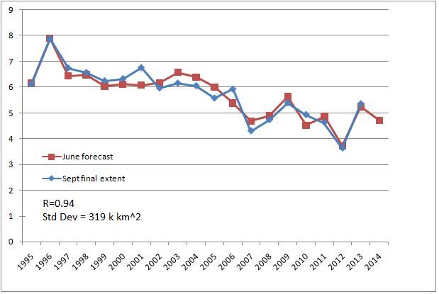
Dekker (Public), 4.70 (+/- 0.32), Statistical
My projection method to estimate September sea ice extent is based on an estimate of how much heat the Northern Hemisphere absorbs during spring and early summer. I found that Northern Hemisphere land snow cover (in March, April, May and June) as well as an estimate of June 'melting ponds and polynia' (June extent - June area) shows particularly strong correlation with Sept sea ice extent, as shown in the graph at:
http://i1272.photobucket.com/albums/y396/RobDekker/June-14_zps7336859b.jpg?t=1404334698
It specifically shows a very low standard deviation on the prediction of just 319 k km2. With my submission I hope to raise some awareness of the importance of loss of land snow cover in spring on Arctic sea ice melt in summer, a correlation which I think has been underrepresented in models and media articles alike.
Kapsch et al, 4.75 (+/- 0.62), Statistical
For the prediction of the September sea-ice extent we use a simple linear regression model that is only based on the atmospheric water vapor in spring (April/May). Thereby we assume that the spring atmospheric conditions, more precisely the greenhouse effect associated with the water vapor in the atmospheric column, are important for the seasonal prediction of the September sea-ice extent.
Stroeve et al, 4.76 (3.66-5.66), Statistical
Our July Outlook contribution represents a slight reduction in the predicted September extent from the June Outlook. As before, we use the survival of ice of different ages to statistically predict the 2014 minimum and use the last 5 years of survival rates as a predictor for this summer. This gives an average estimate of 4.76 ± 0.79 106 km2, and a range from the summer with the lowest (2012) and highest (2009) survival rates within the last 5 years of 3.66 106 km2 to 5.25 106 km2.
Naval Research Lab GOFS, 4.8 (+/- 0.4), Modeling
The Global Ocean Forecast System (GOFS) 3.1 was run in forecast mode without data assimilation, initialized with a June 1, 2014 analysis, for ten simulations using archived Navy atmospheric forcing fields from 2004-2013. The mean minimum ice extent in September, averaged across all ensemble members and corrected for forward model bias is our projected ice extent. The GOFS 3.1 outlook for September minimum ice extent is 4.8 Mkm2 ± 0.4 Mkm2.
Zhang and Lindsay, 4.80 (+/- 0.4), Modeling
Our seasonal prediction focuses not only on the total Arctic sea ice extent, but also on sea ice thickness field and ice edge location. We feel that, for all practical and scientific reasons, it is particularly important to improve our ability to predict the ice thickness and the ice edge. Needless to say, this is a difficult goal. However, we hope that our effort would contribute to this goal.
Slater, 4.85 (+/- 0.56), Statistical
I have extended my forecast method to a 90-day lead time so as to forecast all days in September. The method does have a low level of real skill (taken over 1995-2013). Results contain a large uncertainty at this lead time.
Canadian Ice Service, 4.90, Heuristic/Statistical (No change from June forecast.)
Three methods are combined. The first is heuristic forecast based on analyst interpretations of spring conditions. The second method uses a optimal filtering based statistical model, and the third estimate is based on regression models relating September sea ice extent to spring atmospheric and oceanic conditions.
Barthelemy et al, 5.0 (4.3-5.7), Modeling
Our estimate is based on results from ensemble runs with the global ocean-sea ice coupled model NEMO-LIM3. Each member is initialized from a reference run on June 30, 2014, then forced with the NCEP/NCAR atmospheric reanalysis from one year between 2004 to 2013. Our estimate is the ensemble median, and the given range corresponds to the lowest and highest extents in the ensemble.
Bosse (Public), 5.00 (4.6-5.5), Statistical (No change from June forecast.)
The approach with OHC of the year n-1 as the variable with the most important influence on the melting of the year n is a new one AFAIK. The model is plausible: The melting depends on the quantity of heat of the arctic basin and the volume of the existing seaice-volume in the actual year.
Yuan et al, 5.01 (+/- 0.82), Statistical
The Markov model is capable to capture co-variability in the ocean-sea ice – atmosphere system, which is likely the predictable part of variances in sea ice. The model predicts that the Arctic sea ice extent in September 2014 will be 5.01 million square km. Cross-validation skill, measured by the correlation between three-month lead predictions and observations of September ice extent, is 0.72, while the RMS error of predictions is 0.82 million square km.
GFDL/NOAA (Msadek et al), 5.05 (4.63-5.70), Modeling
Our prediction for the September-averaged Arctic sea ice extent is 5.05 million square kilometers, with an uncertainty range going between 4.63 and 5.70 million square kilometers. Our estimate is based on the GFDL CM2.1 ensemble forecast system in which both the ocean and atmosphere are initialized on July 1 using a coupled data assimilation system. Our prediction is the bias-corrected ensemble mean, and the given range corresponds to the lowest and highest extents in the 10-member ensemble. Our model predicts that September 2014 Arctic sea ice extent will be 1.47 million square kilometers below the 1981 to 2010 observed average extent, but will not reach values as low as those observed in 2007 or 2012.
Wu et al, 5.10 (+/- 0.56), Modeling
Our projection using the NCEP CFSv2 with 30-case of June 2014 revised initial conditions (ICs) is:
September monthly average: 5.1 million square kilometers
Uncertainty: 0.56 million square kilometers
Although the uncertainty dropped from the case of May to June IC, it is still much higher than the previous years.
Li and Li, 5.37 (4.76-5.97), Statistical
We used a simple statistic method to do the sea ice extent prediction. The sea ice extent of September has a good correlation with the sea ice extent of Jan to Apr of the same year and the extent of September 3 years ago. Combined the multiple regression method and optimal climate normal method, we derived the sea ice extent of September this year is 5.37 million square kilometers.
Global Weather and Climate Logistics, 5.39, Statistical
Our predictor screening approach predicts slightly more sea ice extent than last year and our anomaly correlation approach predicts nearly the same sea ice extent as last year. Together the eight ensemble statistical forecasts predict 5.39 million square km of pan-Arctic sea ice extent for September, 2014.
Slater (Persistence), 5.50, Statistical
Three different types of persistence forecasting at long lead time. The methods contain no real skill at the 90 day lead time (cf. skill computed by Schroder et al.).
CPOM (Schroeder et al), 5.51 (+/- 0.44), Statistical
We predict the September 2014 ice extent will be 5.5 million km2, close to the level in 2013. The melt-pond area in May and in the beginning of June has been low due to colder air temperatures and thicker ice in the relevant areas of the Arctic compared to the last 5 years.
Wang, 5.9 (+/- 0.33), Modeling
The predicted sea ice extent range from early July initial conditions is (5.9±0.33) million square kilometers.
Additional Regional Outlook
Global Weather and Climate Logistics: Beaufort Sea and Barents Sea, Statistical
A statistical approach to forecast sea ice area anomalies in the Beaufort Sea and the Barents Sea based on the best predictors chosen from eleven surface and atmospheric variables. The predicted anomaly for the Beaufort Sea is -0.09 * 106 km2 (less than 2013) and for the Barents Sea -0.01 * 106 km2 (greater than 2013).
Individual Outlook PDFs
| Attachment | Size |
|---|---|
| Andersen (Same as June)35.96 KB | 35.96 KB |
| Barthelemy et al.241.57 KB | 241.57 KB |
| Blanchard-Wrigglesworth et al.483.28 KB | 483.28 KB |
| Bosse (Same as June)77.04 KB | 77.04 KB |
| Canadian Ice Service50.88 KB | 50.88 KB |
| Cawley (Same as June)58.56 KB | 58.56 KB |
| CPOM Schroeder et al.48.46 KB | 48.46 KB |
| Dekker42.33 KB | 42.33 KB |
| GFDL NOAA Msadek et al.198.44 KB | 198.44 KB |
| Global Weather Climate Logistics216.33 KB | 216.33 KB |
| Hamilton (Same as June)267.97 KB | 267.97 KB |
| Kapsch et al.60.12 KB | 60.12 KB |
| Kauker et al.187.29 KB | 187.29 KB |
| Kay et al. NCAR50.73 KB | 50.73 KB |
| Li and Li245.48 KB | 245.48 KB |
| Meier1.22 MB | 1.22 MB |
| Morison47.5 KB | 47.5 KB |
| NRL ACNFS501.91 KB | 501.91 KB |
| NRL GOFS614.66 KB | 614.66 KB |
| Rennie482.51 KB | 482.51 KB |
| Slater173.63 KB | 173.63 KB |
| Slater Persistence118.4 KB | 118.4 KB |
| Stroeve et al.205.05 KB | 205.05 KB |
| Suckling (Same as June)107.2 KB | 107.2 KB |
| Wang90.08 KB | 90.08 KB |
| Wu et al.189.7 KB | 189.7 KB |
| Yuan et al.77.02 KB | 77.02 KB |
| Zhang and Lindsay380.58 KB | 380.58 KB |
| Peterson et al. (Same as June; added after Outlook report was drafted)133.29 KB | 133.29 KB |
| NASA GMAO Cullather et al. (Same as June; added after Outlook report was drafted)2.56 MB | 2.56 MB |
| Attachment | Size |
|---|---|
| Blanchard-Wrigglesworth et al.483.28 KB | 483.28 KB |
| Global Weather Climate Logistics783.63 KB | 783.63 KB |
| Zhang and Lindsay380.58 KB | 380.58 KB |
 for September 2014 sea ice extent (labels on the bar graph are rounded to the tenths for readability. Refer to the Individual Outlooks at the bottom of this report for the full details of individual submissions).")