
Outlook Report
Summary
Thank you to the groups that sent outlooks to the 2016 July report. We received 37 total Outlooks; 36 pan-Arctic (3 of which also provided Alaska-regional outlooks), and one additional regional-only outlook. Five contributions included gridded fields.
The writing of this July Outlook report was led by Cecilia Bitz and Ed Blanchard-Wrigglesworth (U. of Washington), with contributions from the rest of the SIPN leadership team.
This month the median pan-Arctic extent Outlook for September 2016 sea ice extent is 4.3 million square kilometers (essentially unchanged from June) with quartiles of 4.1 and 4.6 million square kilometers (See Figure 1 in the full report, below). If the median Outlook should agree with the observed estimate come September, this year would be the third lowest September in the satellite record. The spread in the Outlook contributions narrowed slightly from June to July, with an overall range this month of 3.6 to 5.2 million square kilometers.
The full range of Outlooks submitted this month lies within the range of the 10 lowest years of sea ice extent in the observational record. No Outlook is predicting a new record this year, despite the warm winter, record low extents for every month in 2016 except March, and evidence of thin ice in spring. Does this mean it won't be a record? Meteorological conditions suggest not, as surface temperature over the central Arctic has been near normal in the last month and forecasts of atmospheric circulation for the next few weeks suggest near normal surface temperature in the near future. At the same time, the subpolar seas are warmer than average and the land surrounding the Arctic Ocean has been warm and both are projected to continue to be warm in August and September. Finally, we note that no Outlook predicted a record low in 2012 either, and as a whole, the Outlooks tend to be miss the extreme low and high years compared to the long-term trend.
The 3 Alaskan-Regional Outlooks of September sea ice extent (which includes the Bering, Beaufort, and Chukchi seas as defined in the 2015 Call for Outlooks) were 0.25, 0.7 and 0.87 million square kilometers. The observed September extent in this region over the last decade has a median of 0.46 and quartiles of 0.39 to 0.73.
Among the pan-Arctic Outlooks from 14 dynamic models, the median prediction is 4.5 million square kilometers, with quartiles of 4.1 and 4.8 million square kilometers. The 17 statistical contributions have a smaller median, at 4.3 million square kilometers, and narrower spread, with quartiles of 4.1 and 4.6 million square kilometers.
A section on predicted spatial fields includes discussion on sea ice probability (SIP) submitted from 5 models. A section on current conditions shows the last two months are characterized by relatively normal atmospheric conditions over the Arctic Ocean, but warmer than normal conditions over the subpolar seas and land around the Arctic Ocean. Seasonal climate forecasts indicate continued above normal temperatures in the more southern regions, with especially high temperatures in the Kara and Barents seas.
Overview
As in recent years, the overwhelming majority of submission this month used quantitative methods, of which 17 used statistical methods and 14 used dynamical models. Among the dynamic models, 9 are fully-coupled (with sea ice, ocean and atmosphere components) and 5 are ice-ocean only. We received 3 heuristic contributions (2 from informal polls) and 2 from mixed-methods.
What is a fully-coupled model?
As in June 2016, the median Outlook is higher for dynamical models than for statistical methods, this month by 0.2 million square kilometers (see Figure 2). The range of the Outlooks has narrowed among statistical contributions, mainly by reducing the tail of high values that were submitted in June. The distributions of Outlooks from fully-coupled and ice-ocean only models are roughly the same.
The width of the distribution of Outlooks remains narrower for the second month in a row compared to last year: the interquartile spread across all types of contributions is 0.5 million square kilometers, which is a decrease by about 60% since last year.
For the first time, we received Outlooks for Alaskan-regional sea ice extent, and we hope to expand our reporting on regional Outlooks in future years. The 3 we received are for 0.25, 0.7 and 0.87 million square kilometers, the two higher values are from dynamic models and the third is from a statistical method. The range of these 3 Outlooks is just slightly narrower than the spread of the observed September extent in this region for the last decade.
 for September 2016 sea ice extent.")
Download a high-resolution version of Figure 1.

Comment On Dynamical Modeling Contributions
2016 Modeling Contributions at a Glance
For the July report, we received 14 June SIO submissions from dynamical models: 5 from ice-ocean models forced by atmospheric reanalysis or other atmospheric model output (in green in Figure 3) and 9 from fully coupled general circulation models (in blue in Figure 3). Four fully coupled models re-submitted their June forecasts. The median extent predicted by the models in July is 4. 51 million square kilometers (mean: 4.45 million square kilometers), close to the June Outlook values (4.58 million square kilometers and 4.43 million square kilometers, respectively)
Decomposition of the Spread in the 2016 Model Predictions
Repeating the analysis the spread of Outlook submissions from the June report, the spread among individual models (the dots in Figure 3) amounts to 0.54 million square kilometers, which is similar to the spread among model outlooks seen in the June submissions (0.56 million square kilometers). The mean uncertainty of individual model submissions is 0.53 million square kilometers, only slightly lower than the June value (0.58 million square kilometers).
To conclude, as we found last year, on average there is no substantial evolution in Outlooks submitted between June and July.
 and from all other methods (labeled in grey). The values for Outlooks submitted in July are in black (June submissions are in gray). An asterisk by the forecasters' name indicates the same June forecast has been submitted for July. The dots are the Outlook themselves and the intervals are the uncertainty ranges provided by the groups. Definitions of uncertainty were left to the discretion of the groups themselves, and should therefore be compared with caution. The middle dashed horizontal line is the median of the outlooks from dynamical modeling groups. The lower dashed horizontal line is the lowest bound and the upper line is the largest bound when all dynamical modeling contributions are considered. Figure courtesy of Ed Blanchard-Wrigglesworth.")
Comment On Prediction Maps/Gridded Fields
For the July report, we received 5 submissions of sea ice probability (SIP) and one of ice-free date (IFD). SIP is defined as the fraction of ensemble members in an ensemble forecast with September ice concentration in excess of 15%. IFD is the date in the melt season at which the ice concentration at a given location first drops below 15%.
 from 5 dynamical models, the mean of the 5, and the standard deviation across the 5 SIP forecasts. NRL IO corresponds to Metzger (NRL) and AWI to Kauker in Figure 3. Figure courtesy of Ed Blanchard-Wrigglesworth.")
As was seen in the June submissions, models tend to agree better in the Atlantic/European sector of the Arctic compared to the East Siberian/Alaskan sector this year, as indicated by the standard deviation in SIP. The MetOffice and NOAA forecast of SIP agree on low ice cover in the Beaufort Sea. However the NRL IO model suggests the opposite, and the GFDL model is in between. Post-processing of the SIP forecast could improve this consistency, but at this time we lack an adequate archive of forecasts in past years to apply post processing.
The July model mean SIP is quite similar to the June model mean SIP. However, larger differences can be seen between the two months in the individual models' SIP forecasts (see Figure 5).
 forecasts between the July and June calls for the 4 dynamical models that submitted SIP forecasts in both calls. The model-mean difference panel shows the difference in model-mean SIP for these 4 models between July and June. Figure courtesy of Ed Blanchard-Wrigglesworth.")
Current Conditions
Following the record warm Arctic winter, the lowest sea ice extent at the seasonal maximum in the satellite era, and the lowest ice extent in the months of May and June; the current sea ice cover remains below normal (see Figures 6a and 6b).
The recent atmospheric circulation has driven near normal surface air temperatures (see Figure 7) over much of the central Arctic Ocean (normal compared to a 1981-2010 climatology) in the last two months. Temperatures over the Barents and Kara are noteworthy exceptions, consistent with the extraordinarily low winter and spring sea ice coverage in these seas this year.
The subpolar seas and land surrounding the Arctic Ocean have been mostly warmer than normal (see Figure 7) in the past two months. The pattern over North America is typical of winter conditions during an El Nino event in the tropical Pacific. The associated thinner snow depths could be linked to the warmer spring and summer this year. Note that the warming in the eastern tropical Pacific with El Nino is dissipating rapidly and cooler waters prevail at the equator now.
The warm land and subpolar seas can be seen at the local scale in Barrow, AK, and Longyearbyen, Norway. Both sites experienced much higher temperatures than normal (Figure 8).

Figure 6a images from: http://www.iup.uni-bremen.de:8084/databrowser.html#AMSR2
 and standard deviation (gray). From the NSIDC Arctic Sea Ice News and Analysis.")
Figure 6b image from: http://nsidc.org/arcticseaicenews/charctic-interactive-sea-ice-graph
 averaged from mid-May to mid-July in Arctic and global projections. The Arctic air temperature anomaly is similar throughout the lower troposphere (not shown).")
Figure 7 image from: http://www.esrl.noaa.gov/psd/cgi-bin/data/composites/printpage.pl

Figure 8 upper image from: http://www.cpc.ncep.noaa.gov/products/global_monitoring/temperature/tn7…
Figure 8 lower image from: http://www.yr.no/place/Norway/Svalbard/Longyearbyen/statistics.html
The mean sea level pressure (SLP) in the Arctic over the last month has been markedly low over the central Arctic (see Figure 9), which in the summer tends to result in cooler, cloudier conditions that slow down ice melt. In contrast, SLP has been higher over the Kara sector, which may have contributed to the large current negative anomalies in sea ice concentration in that region of the Arctic. In terms of wind conditions, weak, southerly mean winds over the Fram Strait would presumably have reduced ice export out of the Arctic. In contrast, mean SLP in the previous month was generally higher over most of the Arctic, with a weak low over the Kara and Laptev seas, and weak northwesterly winds over the Fram Strait. The projection of 500mb geopotential height (see Figure 10) for the remainder of July continues the June-to-early July SLP pattern (see Figure 9) with support for low SLP over the Pacific Arctic.

Figure courtesy of Ed Blanchard-Wrigglesworth with data from http://www.yr.no/place/Norway/Svalbard/Longyearbyen/statistics.html
 and anomalies (dotted red contours) for the end of July 2016. Closed contours over the Pacific Arctic support a continued low sea level pressure in that region, similar to Figure 9, which is not supportive of rapid sea ice loss.")
Figure 10 image from: http://www.cpc.ncep.noaa.gov/products/predictions/814day/500mb.php
Seasonal forecasts for the next two months indicate a high probability for continued above average temperature over most of the northern hemisphere in August and September, but average or below average temperatures just off the Siberian coast (see Figure 11). The models contributing to the seasonal forecasts have sea ice components (indeed many of these models also contribute a sea ice Outlook). The high probability of above average temperature in the Barents and Kara seas is a response to the low sea ice cover in the forecasts. To a large extent the probability forecasts in Figure 11 resemble the surface air temperature anomaly of the last two months in Figure 7 in the high latitudes, illustrating the persistence of weak climate anomalies over the sea ice and ocean covered regions throughout the summer months. Summer meteorological current conditions and projections this summer (see Figures 9-11) do not favor extreme mid to late summer sea ice loss in 2016, as occurred in 2007 and 2012, despite low sea ice extents at the beginning of summer.
. Forecasts are issued in July for August (left) and September (right).")
Figure 11 images from: http://www.cpc.ncep.noaa.gov/products/NMME/prob/PROBtmp2m.html
Key Statements/Executive Summaries From Individual Outlooks
The Outlooks are listed below in order of lowest to highest predicted September extent. Extent and uncertainty (in parentheses) values are provided below in units of millions of km2 unless noted otherwise. The individual outlooks can be downloaded as PDFs at the bottom of this webpage.
RASM (Kamal et al.), 3.61 (±0.5), Modeling (fully-coupled)
We used the Regional Arctic System Model (RASM), which is a limited-area, fully coupled climate model consisting of the Weather Research and Forecasting (WRF) model, Los Alamos National Laboratory (LANL) Parallel Ocean Program (POP) and Sea Ice Model (CICE) and the Variable Infiltration Capacity (VIC) land hydrology model (Maslowski et al. 2012; Roberts et al. 2014; DuVivier et al. 2015; Hamman et al. 2016). WRF and VIC are configured on a polar stereographic grid, using the same grid at 50-km resolution, and POP and CICE sharing a rotated spherical grid at 1/12o (~9 km). In this contribution we present the results of a 3-member ensemble.
The three ensemble members (EM) were initialized 12 hours apart, starting on July 1 at 0000 (#1), then at 1200 (#2) and on July 2 at 0000 (#3), using the NCEP version 2 Coupled Forecast System model (CFSv2) seasonal forecast output through September. The National Centers for Environmental Prediction (NCEP) Climate Forecast System Reanalysis (CFSR) data were used for atmospheric forcing along WRF lateral boundaries from 1979 until the respective initialization date and time. In addition, planetary-scale temperature and wind fields were spectrally nudged beginning ~500 hPA with a strength of zero and linearly ramped up to 0.0003 s-1 at the top of the atmosphere, to constrain the large-scale circulation but still allow for free evolution of the boundary layer states. Raw model sea ice concentration data was processed using a simple linear regression model and satellite derived ice extent to produce bias corrected predictions. For all the ensemble members, we used one regression model using 27 years of past model data and NSIDC Merged SMMR and SSM/I sea ice concentration data to estimate and correct for systematic model bias.
Barthélemy et al., 3.8 (2.6-4.6), Modeling (ice-ocean)
Our estimate is based on results from ensemble runs with the global ocean-sea ice coupled model NEMO-LIM3. Each member is initialized from a reference run on June 30, 2016, then forced with the NCEP/NCAR atmospheric reanalysis from one year between 2006 to 2015. Our final estimate is the ensemble median, and the given range corresponds to the lowest and highest extents in the ensemble.
Met Office, 3.8 (± 0.7), Modeling (fully-coupled)
Using the Met Office GloSea5 seasonal forecast systems we are issuing a model based mean September sea ice extent outlook of 3.8 (± 0.7) million km2
This has been assembled using start dates between 15 Jun and 5 Jul to generate an
ensemble of 42 members.
Ionita and Grosfeld (NSIDC Data), 3.89 (3.23-4.56), Statistical
The forecast scheme for the September sea ice extent is based on a methodology similar to one used for the seasonal prediction of river streamflow (Ionita et al., 2008, 2014). The basic idea of this procedure is to identify regions with stable teleconnections between the predictors and the predictand. The September sea ice extent has been correlated with the potential predictors from previous months, up to 8 months lag, in a moving window of 21 years. For the July report we have applied the same analysis for two different sea ice extent data sets: 1) Bremen University (IUP) and 2) National Snow & Ice Data Center (NSIDC). Theses indices differ from month to month by up to 0.6 million km2 due to different retrieval algorithms, special resolutions and different coast line representations. Hence, especially during the summer melting season a different variability is detected, leading to slightly different stability maps of the climatological variables. September 2016 Sea Ice extent based on Bremen University data: 4.25 million km2. Lower uncertainty bound: 3.53 million km2. Upper uncertainty bound: 4.97 million km2. September 2016 Sea Ice extent based on NSIDC data: 3.89 million km2. Lower uncertainty bound: 3.23 million km2. Upper uncertainty bound: 4.56 million km2.
Kay, Bailey, and Holland (NCAR/CU), 3.91 (Std dev = 0.45), Heuristic (Same as June)
An informal pool of 27 climate scientists in early June 2016 estimates that the September 2016 ice extent will be 3.91 km2 (stddev. 0.45, min. 3.14, max. 4.80). Since its inception in 2008, the NCAR/CU sea ice pool has easily rivaled much more sophisticated efforts based on statistical methods and physical models to predict the September monthly mean Arctic sea ice extent (e.g. see appendix of Stroeve et al. 2014 in GRL doi:10.1002/2014GL059388 ; Witness the Arctic article by Hamilton et al. 2014). We think our informal pool provides a useful benchmark and reality check for Sea Ice Prediction efforts based on more sophisticated physical models and statistical techniques.
Morison, 4.0, Heuristic (Same as June)
I had conversations with Axel Schweiger and others following the Seasonal Ice Zone Reconnaissance Surveys (SIZRS) flights during third week of June 2016, who observed some melting but no big ponds as yet. There was open water on and south of 150W, 72N, which puts the ice retreat edge a bit earlier than seen recently. Ice was solid from 74N to 75N with more leads at 76 N, which seems similar to early season patterns seen in recent years that have and intermediate region of pretty solid conditions somewhere south of the Beaufort Gyre center. Usually more winter snow in the Central Arctic has seemed to indicate less September sea ice extent. But, with no spring observations from the North Pole Environmental Observatory in the central Arctic ocean in 2016 I don’t know what the snow conditions were like in that region this year. The winter Arctic Oscillation index was about the same as for 2011 and a similar deviation below the long- term tend would suggest a 2016 minimum extent of 4.2 million km2. This is pretty squishy, but given the current extent and ice conditions in the Beaufort Sea, I think this year’s September average will be about 4 million km2.
NMEFC of China (Li and Li), 4.02 (3.10-4.57), Statistical
We predict the September monthly average sea ice extent of Arctic by statistic method and based on monthly sea ice concentration and extent from National Snow and Ice Data Center. The result shows that the Sep. ice extent of 2016 will be less than in 2015.
NOAA/NCEP/EMC (Wu and Grumbine), 4.09 (Std dev = 0.54), Modeling (fully-coupled)
The projected Arctic minimum sea ice extent from the NCEP CFSv2 model with revised CFSv2 May and June initial conditions (ICs) using 61-member ensemble forecast is 4.09 million km2 with a standard deviation (SD) of 0.54 million km2.
Dekker (Citizen Scientist/Public), 4.1 (Std dev = 0.34), Statistical
My projection is based on an estimate of how much heat the Northern Hemisphere absorbs during spring and early summer. I use three variables (land snow cover, ice concentration, ice area) that are available in June, in a formula which shows particularly strong correlation with Sept sea ice extent. Regressed over the 1992 - 2015 period, the formula projects 4.1 M km^2 for September 2016, with a standard deviation of only 340 k km2.. Past performance of this June forecast method for September ice extent over the past 24 years shown in a graph here. The interesting finding is that the June land snow cover signal is clearly present in the September ice extent numbers.
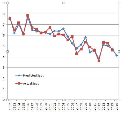
Bosse (Citizen Scientist/Public), 4.1 (±0.43), Statistical (Same as June)
Just as in the two years before I calculate the value for the September-minimum of the arctic sea ice extent of the year n (NSIDC monthly mean for September) from the Ocean Heat Content (0…700m depth) northward 65°N during JJAS of the year n-1. After 2006 the lower sea ice volume of the Februaries also impacts the minimum extent. For the physical explanation see https://www.arcus.org/files/sio/23220/bosse_july2015.pdf .
Petty (NASA-GSFC/UMD), 4.12 (±0.30), Statistical
Based on an analysis of June sea ice concentration data provided by the NSIDC (NASA Team), I forecast a 2016 September Arctic sea ice extent of 4.12 +/- 0.30 million km2. This is lower than the observed ice extent in 2015 (4.63 M km2) and is lower than the extent expected from persistence of the long-term linear trend (4.66 M km2). The forecast does not suggest a new record low September extent will be reached in 2016 (lower than the 3.62 M km2 observed in 2012).
The forecast model uses past sea ice concentration data to find regions of predictive importance for September sea ice extent. The ice concentration in these regions are given more weight in forecasting future sea ice extent. For the 2016 forecast, the strong declines in the southern Beaufort Sea, and the Barents/Kara seas appear to dominate the low forecast, countered somewhat by a small positive anomaly in the Laptev Sea.
Note that a May forecast was produced (not submitted to the SIO) which suggested a lower extent (3.81 +/- 0.40 M km2). However, the skill of the May forecast is lower than the June forecast. The small recovery in sea ice through June appears to suggest a new record is unlikely. The variance of a forecast using linear regression is often biased low, however, so a new record low is still plausible and perhaps outside the scope of this simple model. Uncertain dynamics through summer are also a crucial missing factor, of course.
Hamilton, 4.14 (2.9-5.3), Heuristic (Same as June)
At the Polar Prediction Workshop in May, we carried out an informal poll asking participants for their personal guess about the extent of Arctic sea ice in September 2016. Thirty-five people responded with answers ranging from 2.9 to 5.3 km2 (see Figure 1 in contribution). The lowest prediction would set a new historical record, far below the previous low point of 3.62 set in 2012. The highest prediction would simply mark a return to the 2014 level, which is well below any observations before 2007. So no one is expecting an Arctic sea ice “recovery.” The average among these 35 informal predictions is 4.14 19 km2, which would make September 2016 the second-lowest extent we have seen.
Ionita and Grosfeld (IUP Bremen Data), 4.25 (3.53-4.97), Statistical
The forecast scheme for the September sea ice extent is based on a methodology similar to one used for the seasonal prediction of river streamflow (Ionita et al., 2008, 2014). The basic idea of this procedure is to identify regions with stable teleconnections between the predictors and the predictand. The September sea ice extent has been correlated with the potential predictors from previous months, up to 8 months lag, in a moving window of 21 years. For the July report we have applied the same analysis for two different sea ice extent data sets: 1) Bremen University (IUP) and 2) National Snow & Ice Data Center (NSIDC). Theses indices differ from month to month by up to 0.6 million km2 due to different retrieval algorithms, special resolutions and different coast line representations. Hence, especially during the summer melting season a different variability is detected, leading to slightly different stability maps of the climatological variables. September 2016 Sea Ice extent based on Bremen University data: 4.25 million km2. Lower uncertainty bound: 3.53 million km2. Upper uncertainty bound: 4.97 million km2. September 2016 Sea Ice extent based on NSIDC data: 3.89 million km2. Lower uncertainty bound: 3.23 million km2. Upper uncertainty bound: 4.56 million km2.
Cawley, 4.27 (±1.15), Statistical (Same as June)
This is a purely statistical method (Gaussian Process, related to Kriging) to estimate the long-term trend from previous observations of September Arctic sea ice extent. As this uses only September observations, the prediction is not altered by observations made during the Summer of 2016.
Canadian Ice Service, 4.3 (Avg of 4.1, 4.3, 4.6), Mixed Method
Environment Canada’s Canadian Ice Service (CIS) is predicting the 2016 minimum Arctic sea extent at 4.3 million km2. As with previous CIS contributions, the 2016 forecast was derived by considering a combination of methods: 1) a qualitative heuristic method based on observed end-of-winter Arctic ice thickness/extent, as well as winter surface air temperature, spring ice conditions and the summer temperature forecast; 2) a simple statistical method, Optimal Filtering Based Model (OFBM), that uses an optimal linear data filter to extrapolate the September sea ice extent time-series into the future and 3) a Multiple Linear Regression (MLR) prediction system that tests ocean, atmosphere and sea ice predictors. Based on winter air temperatures and sea ice extents and thickness, a September 2016 minimum ice extent value of 4.3 million km2 is heuristically predicted. The CIS OFB model predicts 4.1 million km2 and the CIS MLR model predicts 4.6 million km2. The average forecast value of the three methods combined is 4.3 million km2.
Meier (NASA GSFC Cryo Sciences), 4.30 (±0.63), Statistical
This method applies daily ice loss rates to extrapolate from the start date (June 3) through the end of September. Projected September daily extents are averaged to calculate the projected September average extent. Individual years from 2006 to 2015 are used as well as averages over 1981 to 2010 and 2006 to 2015. The 2006 to 2015 average daily rates are used to estimate the official submitted estimate.
The predicted September average extent for 2016 is 4.30 (±0.63) million km2. The minimum daily extent is predicted to be 4.19 (±0.62) million km2 and occur on 16 September. The large range of estimates reflects the large variability in ice loss rates over the final three months of the melt season. Based on the last ten years, there is a 20% chance that 2016 will be lower than the current record low extent of 2012.
Arbetter and Potts, 4.31 (3.52-4.47), Statistical
This method is based on the Arctic Regional Ice Forecast System (Drobot et al., International Journal of Climatology, 2009) with additional modifications done by Arbetter at National Ice Center; followed by rewriting and parallelizing the code done by Potts. It uses sea ice, sea level pressure (NCEP), 2-meter surface air temperature (NCEP), and cumulative freezing degree days. 10 years of data are used to establish correlations between conditions at the start week and forecast week. Forecasts are done for 12-16 weeks in the future to cover melt and refreezing.
AWI Consortium (Kauker et al.), 4.32 (±0.30), Modeling (ice-ocean)
We estimate a monthly mean September sea-ice extent of 4.32 +- 0.30 million km2. Sea ice-ocean model ensemble run initialized through assimilation of sea-ice/ocean observations (CryoSat-2 ice thickness, OSI SAF sea ice concentration and SST, and University of Bremen snow depth) in March and April.
Lamont (Yuan et al.), 4.33 (RMSE = 0.61), Statistical
A Linear Markov model is used to predict monthly Arctic sea ice concentration at all grid points in the pan Arctic region. The model is a stochastic linear inverse model that is built in the multi-EOF space and is capable to capture the co-variability in the ocean-sea ice-atmosphere system. September pan Arctic sea ice extent is calculated from predicted sea ice concentration. The model predicts that large negative sea ice concentration anomalies (< -40%) will occur in the Beaufort Sea, Chukchi Sea, Laptev Sea, Kara Sea and
Barents Sea in September 2016. The September mean pan Arctic sea ice extent will be 4.33 million km2.
UAF (Brettschneider, Walsh, and Thoman), 4.36 (4.00-5.52), Statistical
The forecast is based on an analog system in which the years with the atmospheric circulation most similar to 2016 (through June) are identified. The five best analog years are chosen from the 1949-2015 period. The departures of September sea ice from the trend line are averaged for those five years, and that average is our forecast (departure from trend line) for 2016.
FIO-ESM (Qiao et al.), 4.36 (±0.59), Modeling (fully-coupled)
Our prediction is based on FIO-ESM with data assimilation. The prediction of September pan-Arctic extent in 2016 is 4.36 (+/-0.59) million km2. 4.36 and 0.59 million km2 is the average and one standard deviation of 10 ensemble members, respectively.
CNRM (Chevallier et al.), 4.39 (3.45-5.03), Modeling (fully-coupled)
CNRM outlook is based on the operational seasonal forecast issued by Météo France in early July 2016 with the System 5 (component of the European multi-model EUROSIP). Mean September sea ice extent outlook is 4.39 million km2 (ensemble mean of 51-member initialized during the 2 weeks before 1 July and perturbed using stochastic perturbations).
Slater (SPIE), 4.4 (±0.75), Statistical
I have extended my model prediction out to a lead time of 85 days. The method is effectively the same as my “standard” 50 day forecast (http://cires.colorado.edu/~aslater/SEAICE/). At 85 days the method does actually have skill, when measured over the period 1995-2013 and applying a similar skill metric to that used in Schroder et al. 2014. The skill level is only of order 0.10-0.15, but it is real skill nonetheless. (Compare that to an anomaly persistence forecast which has zero skill at this lead time.)
Sun (Citizen Scientist/Public), 4.48 (4.06-4.899), Mixed Method
The forecast model is based on my own global surface radiation model and uses arctic sea ice albedo and land albedo to calculate daily sea ice area and volume losses. The albedo values are obtained from extent/area ratios and northern hemisphere snow cover. The average error for the 2007-2015 period is 4.9% or 0.154 million km2 for daily minimum sea ice area. The final average September extent value is calculated by average ratios of past years.
Slater (Multi-Persistence), 4.53 (Avg: 4.95, 5.06, 3.59), Statistical
Persistence can be computed in several ways. I have looked out to Sept. for the sake of comparison and as a very basic benchmark.
- 1) Daily anomaly persistence at 112 days lead time (so that I can go all the way to Sep 30th), then compute mean for Sept = 4.95
- 2) Persist the absolute anomaly from May to Sept (using NSIDC monthly value, not mean of daily). Sept = 5.06
- 3) Persist the standard normal deviate from May to Sept (using NSIDC monthly). Labeled as "Variance Persistence". Sept = 3.59
None of these methods have true skill at this long lead time. For April-June the daily persistence at 85-day lead time looks like a nice forecast (and is giving better results than a 50-day lead time), however, this is pure coincidence. These methods are different from the “damped persistence” that Ed Blanchard-Wriggleswoth calculates (as I have no damping mechanism built in) …. I/we should throw that one in there as well.
Kaleschke, 4.6 (±0.9), Statistical
I provide a simple statistical estimate for the September sea ice extent based on the total sea ice extent measured on July 11: 4.6±0.9. A discrepancy emerged between the uncertainty of the statistical regression and the melt scenario projections. Because of the low ice concentrations seen in the Central Arctic Basin I consider a 2012-like melt scenario still a reasonable possibility. I had to increase the confidence interval to 5σ to obtain a better match of the uncertainty given by the regression and the different scenarios based on the ice extent loss observed in previous years.
For updates follow me on Twitter @seaice_de.
Jin (IARC), 4.62, Modeling (ice-ocean) (Same as June)
A coupled ice-ocean model (POP-CICE) forecast of the September sea ice extent minimum. The Model is initialized with PHC data and runs from 1958‐2009 with CORE 2 forcing, 2010-2016 with GFDL IPCC atmospheric model output. Since there is only one run, we cannot provide uncertainties.
Wang and Collow, 4.63 ± 0.25, Modeling (fully coupled)(Same as June)
The contribution here includes (1) Monthly September sea ice extent, (2) Monthly September sea ice extent error estimate, and (3) Date of September minimum. We will try to add other additional/optional items for July and August reports. Used CFSv2pp dynamical model; Twenty ensemble members are used. The ensemble members are generated from 5 initial dates (8th - 12th of May at 00Z) with four runs from each initial date. The four runs from each initial date include a control run initialized from CFSR and three additional runs with perturbed initial conditions.
UTokyo (Kimura et al.), 4.68, Statistical
Monthly mean ice extent in September will be about 4.68 million km2. Our estimate is based on a statistical way using data from satellite microwave sensor. We used the ice thickness in December, ice movement from December to April, and ice concentration during June 20-25. Predicted ice concentration map from July to September is available in our website. On the Russian side, sea ice in the Laptev Sea is expected to retreat quickly. On the other hand, sea ice in the East Siberian Sea is likely to retreat slowly. The ice retreat in the East Siberian Sea will be late compared with the last year because the area is covered by thicker ice piled up by the winter convergence of sea ice. On the Canadian side, sea ice in summer is expected to be thin and retreat more quickly than the last year.
GFDL NOAA (Bushuk et al.), 4.70 (4.22-4.99), Modeling (fully-coupled)
Our July 1 prediction for the September-averaged Arctic sea-ice extent is 4.70 million km2, with an uncertainty range of 4.22-4.99 million km2. Our prediction is based on the GFDL-FLOR ensemble forecast system, which is a fully-coupled atmosphere-land-ocean-sea ice model initialized using a coupled data assimilation system. Our prediction is the bias-corrected ensemble mean, and the uncertainty range reflects the lowest and highest sea ice extents in the 12-member ensemble.
NRL-atm-ocn-ice, 4.8 (4.4-5.3), Modeling (fully coupled)(Same as June)
The projected Arctic minimum sea ice extent from the Navy’s global coupled atmosphere-ocean-ice modeling system based on May 2016 initial ice conditions is 4.8 km2. This projection is the average of an 11-member ensemble. The range of the ensemble is 4.4 to 5.3 km2. Note that our ensemble range does not represent a full measure of uncertainty, and the system is currently in a development stage.
Kondrashov, 4.97 (Std dev = 0.2), Statistical
This contribution relies on data-driven approach to predict sea ice conditions over the Pan-Arctic region. The prediction model is obtained by data-adaptive decomposition and inverse modeling of Multisensor Analyzed Sea Ice Extent – Northern Hemisphere (MASIE-NH) dataset.
Zhang and Schweiger, 5.0 (±0.6), Modeling (ice-ocean)
Driven by the NCEP CFS forecast atmospheric forcing, PIOMAS is used to predict the total September 2016 Arctic sea ice extent as well as ice thickness field and ice edge location, starting on July 1. The predicted September ice extent is 5.0± 0.6 million km2. The predicted ice thickness fields and ice edge locations for July, August, and October 2016 are also presented.
NRL-ocn-ice, 5.2 (4.3-6.0), Modeling (ice-ocean)
The Global Ocean Forecast System (GOFS) 3.1 was run in forecast mode without data assimilation, initialized with June 1, 2016 ice/ocean analyses, for ten simulations using National Centers for Environmental Prediction (NCEP) Climate Forecast System Reanalysis (CFSR) atmospheric forcing fields from 2005-2014. The mean ice extent in September, averaged across all ensemble members is our projected ice extent. The GOFS 3.1 outlook for the 2016 September minimum ice extent is 5.2 million km2 with a range of 4.3 – 6.0 million km2
CPOM (Schroeder, Feltham, Flocco, and Tsamados), 5.2 (±0.44), Statistical
We predict the September ice extent 2016 to be slightly lower than last year. Given the extreme low current sea ice extent and the positive SST anomalies, a stronger decline might be expected. But looking at the May 2016 melt pond fraction in our sea ice simulation, the pond fraction is higher in the Kara Sea, north of Svalbard and in the Fram Strait compared to May 2015 and with a lesser extent to May 2012, but lower in the East Siberian Sea and the Arctic Basin. The weighted Arctic wide mean May pond fraction 2016 is higher than in 2015, but much lower than in 2012. While the ice thickness is generally thinner in May 2016 compared to previous years, the air temperature has been several degrees above the last 10 year mean in the northern North Atlantic and the Beaufort Sea, but colder in the Eastern Siberian Sea and Laptev Sea causing the described melt pond pattern.
NASA Global Modeling and Assimilation Office (Cullather et al.), 5.23 (±3.0), Modeling (full-coupled) (Same as June)
The GMAO seasonal forecasting system predicts a September average Arctic ice extent of 5.23±0.30 km2, about 13 percent greater than the 2015 value. While the initial ice cover is remarkably low in the Barents and Kara seas, the forecast suggests limited reductions in ice extent on the Pacific side of the Arctic as compared with recent years. This is the final year of sea ice forecasts with the current system, a new GMAO seasonal forecasting system will be in place next year.
Individual Outlook PDFs
