
Outlook Report
Summary
Thank you to the groups that sent outlooks to the 2016 August report. We received 40 Outlooks; 39 pan-Arctic (three of which also provided Alaska-regional Outlooks), and one additional regional-only Outlook (ARCUS/editor's note 8/26 - this is a record number of contributions for the Sea Ice Outlook - thank you!). Five contributions included gridded fields.
The writing of this August Outlook report was led by Jim Overland (NOAA) with contributions from the SIPN leadership team.
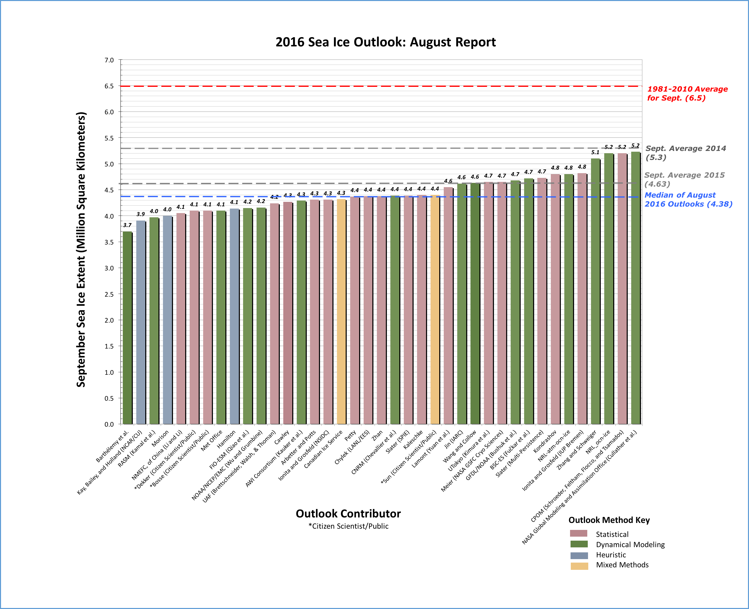
This month the median pan-Arctic extent Outlook for September 2016 sea ice extent is 4.4 million square kilometers (km2) with quartiles of 4.2 and 4.7 million km2, which is slightly higher than July's value (4.3 million km2) (See Figure 1 in the full report, below). If the median Outlook should agree with the observed estimate come September, this year would be the third lowest September in the satellite record. The spread in the Outlook contributions narrowed slightly from July to August, with an overall range this month of 3.7 to 5.2 million km2.
The full range of Outlooks submitted this month lies within the range of the ten lowest years of sea ice extent in the observational record. As in July, no Outlook is predicting a new record this year, despite the warm winter, record low extents for every month in 2016 except March and July, and evidence of thin ice in spring. Current sea ice extent and meteorological conditions suggest a record low is unlikely, as surface temperature over the central Arctic has been near normal in the last two months and forecasts of atmospheric temperatures for the next few weeks indicate average surface temperatures. However, a major storm in the central Arctic during mid- to late August will support continued breakup of the central ice pack. The higher end of the predictions is also unlikely given that the current extent as of 16 August is 5.3 million km2.
Overview
As in June and July 2016, the median Outlook is higher for dynamical models than for statistical methods, this month by 0.2 million square kilometers (km2). The width of the distribution of Outlooks compared to last year remains narrow for the third month in a row: the interquartile spread across all types of contributions is 0.5 million km2 which is a decrease by about 60% since last year.
 for September 2016 sea ice extent.")
Download a high-resolution version of Figure 1.
(A note about accuracy and precision: the numerical values in Figure 1 are rounded to just one decimal place although the height of each bar is determined to two decimal places, this results in a small discrepancy in statistics. The August median rounded to one decimal place is 4.4, to two decimal places it is 4.38.)
. A gray line shows the 2015 observed September extent, for comparison. Figure courtesy of Larry Hamilton")
Comment On Dynamical Modeling Contributions
2016 Modeling Contributions at a Glance
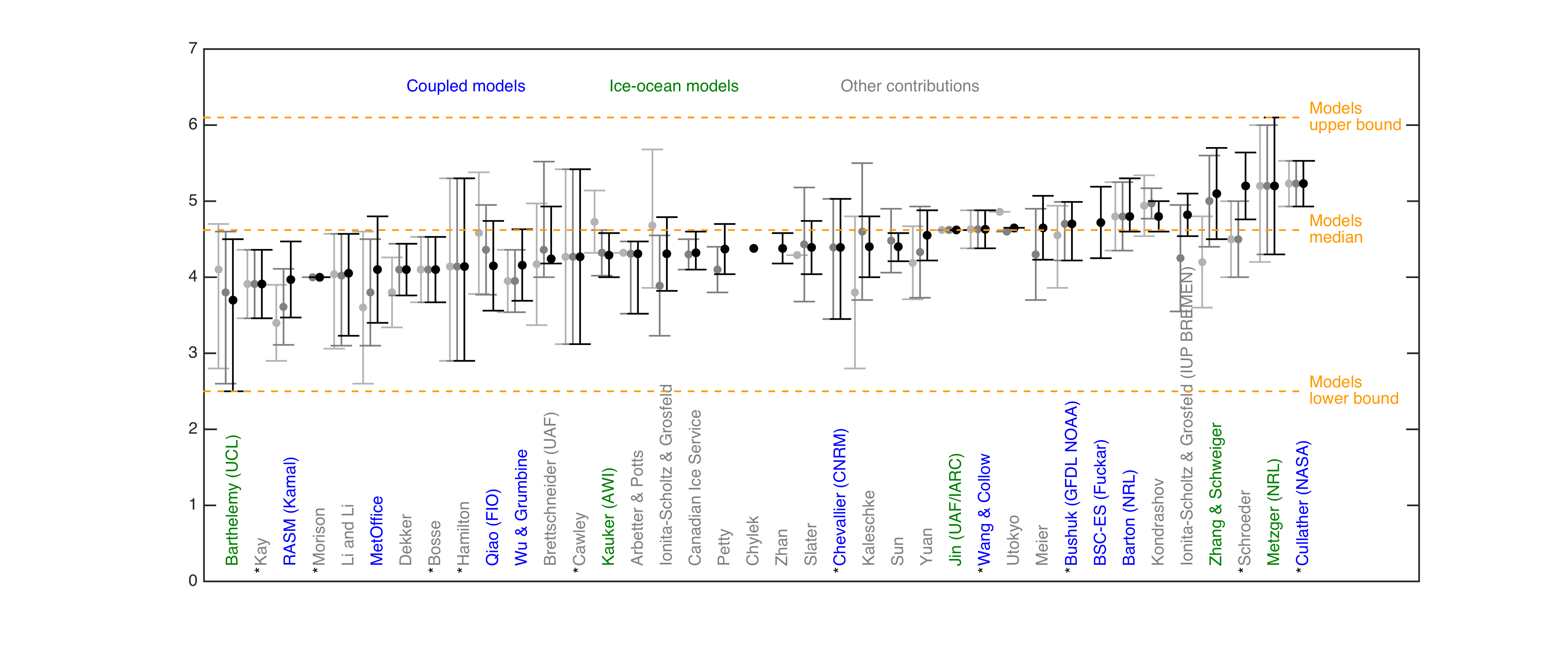
In our August call, we received 15 Sea Ice Outlook (SIO) submissions from dynamical models, five from ice-ocean models forced by atmospheric reanalysis or other atmospheric model output (in green in Figure 3) and ten from fully coupled general circulation models (in blue in Figure 3). Four fully coupled models re-submitted their July forecasts. The median extent predicted by the models in August is 4.62 million km2 (mean: 4.51 million km2), slightly higher than the values for the July and June SIOs.
Decomposition of the Spread in the 2016 Model Predictions
Repeating the analysis of the spread of Outlook submissions from the June and July reports, the spread among individual models (the heavy dots in Figure 3) amounts to 0.49 million km2 which is only slightly lower than the spread among model outlooks seen in the June and July submissions (0.56 million km2 and 0.54 million km2 respectively). The mean uncertainty of individual model submissions is 0.53 million km2, which is the same as the July SIO model uncertainty.
Interestingly, different models' mean forecasts undergo different tendencies from the June SIO to the August SIO. For example, the UCL and FIO SIOs become increasingly smaller, yet the MetOffice and RASM SIOs become increasing larger over the SIO submission period.
 and from all other methods (labeled in grey). The values for Outlooks submitted in August are in black (July submissions are in dark gray and June submissions are in light gray). An asterisk by the forecasters' name indicates the same July forecast has been submitted for August. The dots are the Outlook submissions themselves and the intervals are the uncertainty ranges provided by the groups. Definitions of uncertainty were left to the discretion of the groups themselves, and should therefore be compared with caution. The middle dashed horizontal line is the median of the outlooks from dynamical modeling groups. The lower dashed horizontal line is the lowest bound and the upper line is the largest bound when all dynamical modeling contributions are considered. Figure courtesy of Ed Blanchard-Wrigglesworth.")
Download a high-resolution version of Figure 3.
Comment On Prediction Maps/Gridded Fields
For the August call, we received five submissions of Sea Ice Probability (SIP) and two of ice-free date (IFD). (For definitions of SIP and IFD, see the August call for contributions).
 from five dynamical models, the mean of the five, and the standard deviation across the five SIP forecasts. NRL IO corresponds to Metzger (NRL) in Figure 2. The bottom right panel shows the difference in the model-mean SIP between the August and July SIOs for the five models. Figure courtesy of Ed Blanchard-Wrigglesworth.")
As was seen in the June and July submissions, models tend to agree better in the Atlantic/European sector of the Arctic compared to the East Siberian/Alaskan sector this year, as indicated by the standard deviation in SIP. Uncertainty is particularly high in the East Siberian region, where NRL IO predicts a high chance of ice survival, while NOAA (AWI) predicts a low chance.
 forecasts between the August and July calls for the four dynamical models that submitted SIP forecasts in both calls. The model-mean difference panel shows the difference in model-mean SIP for these four models between August and July. Figure courtesy of Ed Blanchard-Wrigglesworth.")
Compared to the mean July SIP forecast from all five models, August shows slightly higher chances of ice survival along the Siberian coastlines and the Kara sea, and lower in the Beaufort region. However, there is considerable uncertainty across models in the SIP forecast tendency between the July and August SIOs, as was seen earlier between the June and July SIOs (see July report).
Current Conditions
Following the record warm Arctic winter, sea ice had the lowest extent at the seasonal maximum in the satellite era, and the lowest ice extent in the months of May and June; the current sea ice cover remains below normal, but now is greater than the minimum year of 2012 (Figure 6). Much of the central pack remains diffuse with areas of <50 % concentration (Figure 7). In contrast to the past eight years, extensive ice in the Laptev Sea blocks the Northern Sea Route.
The recent atmospheric circulation has driven near average surface air temperatures over much of the central Arctic Ocean (compared to a 1981-2010 climatology) in the last two months. Temperatures over the Barents and Kara are noteworthy exceptions, consistent with the extraordinarily low winter and spring sea ice coverage in these seas this year. (see NSIDC).
 and standard deviation (gray). From the NSIDC Arctic Sea Ice News and Analysis.")
Figure 6 image from: http://nsidc.org/arcticseaicenews/charctic-interactive-sea-ice-graph.

Figure 7 image from: http://www.iup.uni-bremen.de:8084/databrowser.html#AMSR2.
The mean sea level pressure (SLP) in the Arctic over the last month continues to be markedly low over the central Arctic, which results in cooler, cloudier conditions that slow down ice melt. Starting in mid-August, and projected through the end of August, the low pressure has intensified to the second strongest August storm on record after August 2012. Increased winds in 2012 helped to break up the ice pack in that year and contributed to the record minimum extent. A similar wind contribution may also impact 2016, but as seen in Figure 6, the 2016 ice pack has a considerable more extent at this time of year than in 2012. The projection of 500 mb geopotential height (Figure 8) for mid- late August continues to support the strong low SLP August storm pattern. Thus conditions remain unlikely for surpassing the record low September extent of 2012. However, 2016 will remain among the lowest September values recorded during the satellite data record based in part on its initial low extent and thin ice cover in May 2016 and the possible impact of the August storm.
 and anomalies (dotted red/blue contours) for mid-August 2016. Closed contours over the Pacific Arctic indicate a continued low sea level pressure in that region, which is not supportive of rapid sea ice loss.")
Figure 8 image from: http://www.cpc.ncep.noaa.gov/products/predictions/814day/500mb.php.
Comment On Sea Ice Conditions in the Alaska Sector
Three estimates submitted in the August Outlook for sea ice extent in the Alaska box were 0.7, 0.6 and 0.3 million km2 (Chylek, NRL-Ocean, Petty), compared with the 10 year mean of 0.6 million km2.
Through late May, ice conditions in the Alaska sector, both in the Bering and Chukchi Seas had been unusually mild. Freeze-up and coastal ice formation in the southern Bering Sea were delayed by more than two months in some locations and ice thickness in the coastal Chukchi Sea was well below normal (see June report). At Barrow, Alaska, surface melt was well advanced in the last week of May, with extensive ponding and little remnants of snow cover. However, beginning in early June and extending into July, cooler conditions prevailed throughout the Chukchi and Beaufort Seas, bringing melt to a temporary halt. Morison reported that flight observations at the end of June did not show extensive melting yet. In late July, NOAA survey flights (Figure 9) showed extensive sea ice northwest of Barrow. Note that mostly calm conditions and cooler temperatures helped maintain this ice despite its low thickness and ponds having melted through (Figure 9 insert bottom left).
 and remnants of deformed, thicker ice (top left). (Photos courtesy of NOAA Aerial Surveys of Arctic Marine Mammals program)")
With a major cyclone present in mid-August 1000 km north of Barrow and stormier conditions expected in the Chukchi Sea in late August/early September, ice such as that in Figure 9 bottom left is primed for break-up. Advection of warmer ocean water will further accelerate melt. Highly deformed ice (Figure 9, middle right) that forms as a result of ice-pack coastal interaction north of the Alaskan and East Siberian landmass is expected to linger further (see ice tongue visible in Figure 7). Such scattered thick ice has also been advecting into coastal waters off Barrow (Figure 10) and will continue to present a hazard to vessels in the region. Note that the tongue of sea ice in the Chukchi Sea roughly matches the area of largest model uncertainty in the SIP forecasts (Figure 4). Given the importance of this region for ecosystems and maritime activities, it may warrant a closer look at how well the relevant processes are represented in the different models.
For the remainder of the ice season, ice retreat both in the Alaska Arctic and further north will be controlled by the combination of dynamic break-up of floes under the force of strong winds (Such as the major cyclone developing in mid-August –as discussed in the Wunderground blog) and melt of ice floes and fragments. As indicated in the contribution by Schroeder et al., pond extent in the Pacific and High Arctic sectors appears to be less than in 2012 during the previous record minimum (and the occurrence of a major Arctic cyclone that advanced break-up and ice retreat). Hence, we may still not reach or surpass the 2012 ice minimum.
Ocean heat content is another important variable in this context. Sea surface temperatures in the Alaskan Arctic are slightly lower than during 2012 2012 (see the UpTempO website), but Arctic-wide 2012 and 2016 are roughly comparable. If the large cyclone results in a major reduction in ice concentration, storm winds may further mix the ocean heat, which would also promote delays in freeze-up.

For Figure 10, more details and ice observation logs are available on ELOKA’s SIZONet website.
19 August Update: Images of the passage of the major cyclone developing in mid-August and break-up of ice cover are recorded by NSF-AON O-buoys. An animation of the buoy images leading up to the storm is available on the NSF-AON O-Buoy Project movie tab Real-Time Telemetry Monitor. The video will be updated to cover the passage of the storm. Images are taken every 15 minutes with the most recent image available on the NSF-AON O-Buoy Project website.

To view full image sequence of storm passage visit http://obuoy.datatransport.org/monitor#buoy14/movie and advance to last section of image feed.
Key Statements/Executive Summaries From Individual Outlooks
The Outlooks are listed below in order of lowest to highest predicted September extent. Extent and uncertainty (in parentheses) values are provided below in units of millions of km2 unless noted otherwise. The individual outlooks can be downloaded as PDFs at the bottom of this webpage.
Barthélemy et al., 3.7 (2.5-4.5), Modeling
Our estimate is based on results from ensemble runs with the global ocean-sea ice coupled model NEMO-LIM3. Each member is initialized from a reference run on July 31, 2016, then forced with the NCEP/NCAR atmospheric reanalysis from one year between 2006 to 2015. Our final estimate is the ensemble median, and the given range corresponds to the lowest and highest extents in the ensemble.
Kay, Bailey, and Holland (NCAR/CU), 3.91 (Std dev = 0.45), Heuristic (Same as June)
An informal pool of 27 climate scientists in early June 2016 estimates that the September 2016 ice extent will be 3.91 km2 (stddev. 0.45, min. 3.14, max. 4.80). Since its inception in 2008, the NCAR/CU sea ice pool has easily rivaled much more sophisticated efforts based on statistical methods and physical models to predict the September monthly mean Arctic sea ice extent (e.g. see appendix of Stroeve et al. 2014 in GRL doi:10.1002/2014GL059388 ; Witness the Arctic article by Hamilton et al. 2014). We think our informal pool provides a useful benchmark and reality check for Sea Ice Prediction efforts based on more sophisticated physical models and statistical techniques.
RASM (Kamal et al.), 3.97 (±0.5), Modeling
We used the Regional Arctic System Model (RASM), which is a limited-area, fully coupled climate model consisting of the Weather Research and Forecasting (WRF) model, Los Alamos National Laboratory (LANL) Parallel Ocean Program (POP) and Sea Ice Model (CICE) and the Variable Infiltration Capacity (VIC) land hydrology model (Maslowski et al. 2012; Roberts et al. 2014; DuVivier et al. 2015; Hamman et al. 2016). WRF and VIC are configured on a polar stereographic grid, using the same grid at 50-km resolution, and POP and CICE sharing a rotated spherical grid at 1/12o (~9 km). In this contribution we present the results of a 6-member ensemble.
The six ensemble members (EMs) were initialized 6 hours apart, starting on August 1 at: 0000 (#1), 0600 (#2), 1200 (#3), 1800 (#4), and on Augsut 2 at: 0000 (#5), and 0600 (#6), using the NCEP version 2 Coupled Forecast System model (CFSv2) seasonal forecast output through September. The National Centers for Environmental Prediction (NCEP) Climate Forecast System Reanalysis (CFSR) data were used for atmospheric forcing along WRF lateral boundaries from 1979 until the respective initialization date and time. In addition, planetary-scale temperature and wind fields were spectrally nudged beginning ~500 hPA with a strength of zero and linearly ramped up to 0.0003 s-1 at the top of the atmosphere, to constrain the large-scale circulation but still allow for free evolution of the boundary layer states. Raw model sea ice concentration data was processed using a simple linear regression model and satellite derived ice extent to produce bias corrected predictions. For all the ensemble members, we used one regression model using 27 years of past model data and NSIDC Merged SMMR and SSM/I sea ice concentration data to estimate and correct for systematic model bias.
Morison, 4.0, Heuristic (Same as June)
I had conversations with Axel Schweiger and others following the Seasonal Ice Zone Reconnaissance Surveys (SIZRS) flights during third week of June 2016, who observed some melting but no big ponds as yet. There was open water on and south of 150W, 72N, which puts the ice retreat edge a bit earlier than seen recently. Ice was solid from 74N to 75N with more leads at 76 N, which seems similar to early season patterns seen in recent years that have and intermediate region of pretty solid conditions somewhere south of the Beaufort Gyre center. Usually more winter snow in the Central Arctic has seemed to indicate less September sea ice extent. But, with no spring observations from the North Pole Environmental Observatory in the central Arctic ocean in 2016 I don’t know what the snow conditions were like in that region this year. The winter Arctic Oscillation index was about the same as for 2011 and a similar deviation below the long- term tend would suggest a 2016 minimum extent of 4.2 million km2. This is pretty squishy, but given the current extent and ice conditions in the Beaufort Sea, I think this year’s September average will be about 4 million km2.
NMEFC of China (Li and Li ), 4.05 (3.23-4.57), Statistical
We predict the September monthly average sea ice extent of Arctic by statistic method and based on monthly sea ice concentration and extent from National Snow and Ice Data Center. The result shows that the Sep. ice extent of 2016 will be less than in 2015.
Dekker (Citizen Scientist/Public), 4.1 (Std dev = 0.34), Statistical (Same as July)
My projection is based on an estimate of how much heat the Northern Hemisphere absorbs during spring and early summer. I use three variables (land snow cover, ice concentration, ice area) that are available in June, in a formula which shows particularly strong correlation with Sept sea ice extent. Regressed over the 1992 - 2015 period, the formula projects 4.1 M km^2 for September 2016, with a standard deviation of only 340 k km2.. Past performance of this June forecast method for September ice extent over the past 24 years shown in a graph here. The interesting finding is that the June land snow cover signal is clearly present in the September ice extent numbers.
Bosse (Citizen Scientist/Public), 4.1 (±0.43), Statistical (Same as June)
Just as in the two years before I calculate the value for the September-minimum of the arctic sea ice extent of the year n (NSIDC monthly mean for September) from the Ocean Heat Content (0…700m depth) northward 65°N during JJAS of the year n-1. After 2006 the lower sea ice volume of the Februaries also impacts the minimum extent. For the physical explanation see https://www.arcus.org/files/sio/23220/bosse_july2015.pdf .
Met Office, 4.1 (±0.7), Modeling
Using the Met Office GloSea5 seasonal forecast systems we are issuing a model based mean September sea ice extent outlook of 4.1 (± 0.7) million km2. This has been assembled using start dates between 15 Jul and 4 Aug to generate an ensemble of 42 members.
Hamilton, 4.14 (2.9-5.3), Heuristic (Same as June)
At the Polar Prediction Workshop in May, we carried out an informal poll asking participants for their personal guess about the extent of Arctic sea ice in September 2016. Thirty-five people responded with answers ranging from 2.9 to 5.3 km2 (see Figure 1 in contribution). The lowest prediction would set a new historical record, far below the previous low point of 3.62 set in 2012. The highest prediction would simply mark a return to the 2014 level, which is well below any observations before 2007. So no one is expecting an Arctic sea ice “recovery.” The average among these 35 informal predictions is 4.14 19 km2, which would make September 2016 the second-lowest extent we have seen.
FIO-ESM (Qiao et al.), 4.15 (±0.59), Modeling
Our prediction is based on FIO-ESM with data assimilation. The prediction of September pan-Arctic extent in 2016 is 4.15 (±0.59) million km2. 4.15 and 0.59 million km2 is the average and one standard deviation of 10 ensemble members, respectively.
NOAA/NCEP/EMC (Wu and Grumbine), 4.16 (Std dev = 0.47), Modeling
The projected Arctic minimum sea ice extent from the NCEP CFSv2 model with revised CFSv2 May to July initial conditions (ICs) using 92-member ensemble forecast is 4.16 million km2 with a standard deviation (SD) of 0.47 million km2.
UAF (Brettschneider, Walsh, & Thoman), 4.24 (4.18-4.93), Statistical
The forecast is based on an analog system in which the years with the atmospheric circulation most similar to 2016 (through June) are identified. The five best analog years are chosen from the 1949-2015 period. The departures of September sea ice from the trend line are averaged for those five years, and that average is our forecast (departure from trend line) for 2016.
Cawley, 4.27 (±1.15), Statistical (Same as June)
This is a purely statistical method (Gaussian Process, related to Kriging) to estimate the long-term trend from previous observations of September Arctic sea ice extent. As this uses only September observations, the prediction is not altered by observations made during the Summer of 2016.
AWI Consortium (Kauker et al.), 4.29 (± 0.29), Modeling
We estimate a monthly mean September sea-ice extent of 4.29 ±0.29 million km2. Sea ice-ocean model ensemble run initialised through assimilation of sea-ice/ocean observations (CryoSat-2 ice thickness, OSI SAF sea ice concentration and SST, and University of Bremen snow depth) in March and April.
Arbetter and Potts, 4.31 (3.52-4.47), Statistical (Same as July)
This method is based on the Arctic Regional Ice Forecast System (Drobot et al., International Journal of Climatology, 2009) with additional modifications done by Arbetter at National Ice Center; followed by rewriting and parallelizing the code done by Potts. It uses sea ice, sea level pressure (NCEP), 2-meter surface air temperature (NCEP), and cumulative freezing degree days. 10 years of data are used to establish correlations between conditions at the start week and forecast week. Forecasts are done for 12-16 weeks in the future to cover melt and refreezing.
Ionita and Grosfeld (NSIDC), 4.31 (3.82-4.79), Statistical
Sea ice in both Polar Regions is an important indicator for the expression of global climate change and its polar amplification. Consequently, a broad information interest exists on sea ice, its coverage, variability and long term change. Knowledge on sea ice requires high quality data on ice extent, thickness and its dynamics. As an institute on polar research we collect data on Arctic and Antarctic sea ice, investigate its physics and role in the climate system and provide model simulations on different time scales. All this data is of interest for science and society. In order to provide insights into the potential development of the seasonal signal, we developed a robust statistical model based on ocean heat content, sea surface temperature and atmospheric variables to calculate an estimate of the September minimum sea ice extent for every year. This is applied for the year 2016 the first time and we will provide updated results every month for the sea ice outlook report.
For the August report we have applied the same analysis than in previous months for two different sea ice extent data sets:
1) Bremen University (IUP) (http://iup.physik.uni-bremen.de:8084/ssmis/) and
2) National Snow & Ice Data Center (NSIDC) (https://nsidc.org/data/seaice_index/).
Despite the same used climatological data sets, we considered both sea ice extent indices for two different analyses. The indices differ from month to month by up to 0.6 million km2 due to different retrieval algorithms, spatial resolutions and different coast line representations. Hence, especially during the summer melting season a different variability is detected, leading to slightly different stability maps of the climatological variables.
Canadian Ice Service, 4.33 (Avg of 4.1, 4.3, 4.6), Mixed Method (Same as July)
Environment Canada’s Canadian Ice Service (CIS) is predicting the 2016 minimum Arctic sea extent at 4.3 million km2. As with previous CIS contributions, the 2016 forecast was derived by considering a combination of methods: 1) a qualitative heuristic method based on observed end-of-winter Arctic ice thickness/extent, as well as winter surface air temperature, spring ice conditions and the summer temperature forecast; 2) a simple statistical method, Optimal Filtering Based Model (OFBM), that uses an optimal linear data filter to extrapolate the September sea ice extent time-series into the future and 3) a Multiple Linear Regression (MLR) prediction system that tests ocean, atmosphere and sea ice predictors. Based on winter air temperatures and sea ice extents and thickness, a September 2016 minimum ice extent value of 4.3 million km2 is heuristically predicted. The CIS OFB model predicts 4.1 million km2 and the CIS MLR model predicts 4.6 million km2. The average forecast value of the three methods combined is 4.3 million km2.
Petty, 4.37 (±0.33), Statistical
Based on an analysis of July sea ice concentration data provided by the NSIDC (NASA Team), I forecast a 2016 September Arctic sea ice extent of 4.37 +/- 0.33 million km2. This is lower than the observed ice extent in 2015 (4.63 million km2) and is lower than the extent expected from persistence of the long-term linear trend (4.66 million km2). The forecast does not suggest a new record low September extent will be reached in 2016 (lower than the 3.62 million km2 observed in 2012). This forecast is slightly higher than the June forecast submitted to the SIO (4.12 million km2). For the 2016 July forecast, the anomalous declines in the Beaufort and Barents seas are countered by a stronger (than June) positive anomaly in the Laptev Sea.
Chylek (LANL/EES), 4.38, Statistical
For each sea determine the average sea ice decrease between July 20 and September average considering 2006-2015 data. From the “current” state of July 20, 2016 of each sea subtract the average amount with constrain that sea ice extent cannot be negative for any of the seas. Sum over all the seas.
Zhan, 4.38 (±0.2), Statistical
Our statistical model is based purely on the June top-of-atmosphere reflected solar radiation (RSR). It works because the main contribution to the Pan-Arctic June RSR anomaly is the surface albedo variation, especially for the region consisting of the Beaufort Sea and E. Siberian Sea (BESS). Compared to June 2015, MISR shows a significant decrease in RSR over both the south Beaufort Sea and E. Siberian Sea, but an increase in the west Laptev Sea and Chukchi Sea. The area-weighted Pan-Arctic mean June RSR 2016 is lower than that in 2015, but follows the 2002-2015 trend with a slightly positive anomaly. Thus, we estimated the September sea-ice extent 2016 follows its 2002-2015 trend with a slightly positive anomaly.
CNRM (Chevallier et al.), 4.39 (3.45-5.03), Modeling (Same as July)
CNRM outlook is based on the operational seasonal forecast issued by Météo France in early July 2016 with the System 5 (component of the European multi-model EUROSIP). Mean September sea ice extent outlook is 4.39 million km2 (ensemble mean of 51-member initialized during the 2 weeks before 1 July and perturbed using stochastic perturbations).
Slater (SPIE), 4.39 (±0.35), Statistical
This is a 54-day lead time probabilistic forecast, covering all days in September. Exactly how much of the Chukchi and ESS will melt out is uncertain. Did the warm spring impact the thickness more than is visible in current imagery? Since early July, 2016 has been in the vicinity of 2007, 2011 and 2012 extents (but by August the low concentrations of 2012 set the future pattern). Extent is 6.13 at date of issue; 1.74 x 10⁶ million km2 is the difference to the forecast mean. I would be surprised if my forecast was excessively low, though one never knows. The weather will govern the remaining details.
Kaleschke, 4.4 (±0.4), Statistical
I provide a simple statistical estimate for the September sea ice extent based on the total sea ice extent measured in August: 4.4±0.4. Sea ice extent from ADS, projections based on past declines, and statistical regression based on August 8 (x-axis) and Sept (y-axis) scaled to NSIDC monthly values. Uncertainties of the statistical regression are given with 5σ intervals. For updates follow me on Twitter @seaice_de.
Sun (Citizen Scientist/Public), 4.4 (4.21-4.58), Mixed Method
The forecast model is based on my own global surface radiation model and uses arctic sea ice albedo and land albedo to calculate daily sea ice area and volume losses. The albedo values are obtained from extent/area ratios and northern hemisphere snow cover. The average error for the 2007-2015 period is 4.9% or 0.154 million km2 for daily minimum sea ice area. The final average September extent value is calculated with ratios of past years.
Lamont (Yuan et al.), 4.55 (RMSE=0.33), Statistical
A Linear Markov model is used to predict monthly Arctic sea ice concentration at all grid points in the pan Arctic region. The model is a stochastic linear inverse model that is built in the multi-EOF space and is capable to capture the co-variability in the ocean-sea ice-atmosphere system. September pan Arctic sea ice extent is calculated from predicted sea ice concentration. The model predicts that large negative sea ice concentration anomalies (< -40%) will occur in the Beaufort Sea, Chukchi Sea, Laptev Sea, Kara Sea and Barents Sea in September 2016. The September mean total Arctic sea ice extent will be 4.55 million km2.
Jin (IARC), 4.62, Modeling (Same as June)
A coupled ice-ocean model (POP-CICE) forecast of the September sea ice extent minimum. The Model is initialized with PHC data and runs from 1958‐2009 with CORE 2 forcing, 2010-2016 with GFDL IPCC atmospheric model output. Since there is only one run, we cannot provide uncertainties.
Wang and Collow, 4.63 ± 0.25, Modeling (Same as June)
The contribution here includes (1) Monthly September sea ice extent, (2) Monthly September sea ice extent error estimate, and (3) Date of September minimum. We will try to add other additional/optional items for July and August reports. Used CFSv2pp dynamical model; Twenty ensemble members are used. The ensemble members are generated from 5 initial dates (8th - 12th of May at 00Z) with four runs from each initial date. The four runs from each initial date include a control run initialized from CFSR and three additional runs with perturbed initial conditions.
UTokyo (Kimura et al.), 4.65, Statistical
Monthly mean ice extent in September will be about 4.65 million km2. Our estimate is based on a statistical way using data from satellite microwave sensor. We used the ice thickness in December, ice motion from December to April, and ice concentration during July 20-25. Predicted ice concentration map from August 1 to November 1 is available in our website: http://ccsr.aori.u-tokyo.ac.jp/~kimura_n/arctic/2016_e.html
On the Russian side, sea ice in the Laptev Sea is expected to retreat quickly. On the other hand, ice retreat in the East Siberian Sea will be late compared with the last year because the area is covered by thicker ice that was piled up by the winter convergence of sea ice.
Meier (NASA GSFC Cryo Sciences), 4.65 (±0.42), Statistical
This method applies daily ice loss rates to extrapolate from the start date (July 31) through the end of September. Projected September daily extents are averaged to calculate the projected September average extent. Individual years from 2006 to 2015 are used as well as averages over 1981 to 2010 and 2006 to 2015. The 2006 to 2015 average daily rates are used to estimate the official submitted estimate.
The predicted September average extent for 2016 is 4.65 (±0.42) million km2. The minimum daily extent is predicted to be 4.53 (±0.43) million km2 and occur on 16 September. This is a substantial increase over the July projections of 4.30 million square kilometers for the September average and 4.19 million km2 for the minimum daily extent. This change reflects the relatively slow retreat during July. The range of the estimates has dropped by ~33% over July. This is expected because as the time frame shortens, the envelope of the possible extent narrows. However, it is still quite large and indicates that there is a still a large range of possible outcomes due to the large variability in ice loss rates over the final two months of the melt season. Based on the last ten years, there is a <10% chance that 2016 will be lower than the current record low extent of 2012.
GFDL/NOAA (Bushuk et al.), 4.68 (4.00-5.27), Modeling
Our August 1 prediction for the September-averaged Arctic sea-ice extent is 4.68 million km2, with an uncertainty range of 4.00-5.27 million km2. Our prediction is based on the GFDL-FLOR ensemble forecast system, which is a fully-coupled atmosphere-land-ocean-sea ice model initialized using a coupled data assimilation system. Our prediction is the bias-corrected ensemble mean, and the uncertainty range reflects the lowest and highest sea ice extents in the 12-member ensemble.
BSC-ES (Fučkar et al.), 4.72 (Std dev = 0.47), Modeling
We produced September 2016 forecast of Arctic sea ice conditions using coupled climate model (EC-Earth2.3) initialized on May 1st, 2016. This state-of-the-art coupled general circulation model includes dynamic-thermodynamics model of sea ice, LIM2, embedded in NEMO2 ocean model with horizontal resolution of about 1 degree (ORCA1L42). We employ dynamical models for seasonal forecast because they have capability to resolve and predict details of sea ice cover in non-stationary and physically consistent manner.
Slater (Persistence), 4.73 (Avg of 4.86, 4.86, and 4.48), Statistical
Three different types of persistence forecasting at 54-day or 2 month lead time. The methods contain quite reasonable skill at this timescale. Both monthly and daily absolute anomaly persistence give 4.86 million km2.
Kondrashov, 4.8 (Std dev = 0.2), Statistical
Multisensor Analyzed Sea Ice Extent – Northern Hemisphere (MASIE-NH) daily dataset (2006 - June 2016) was used. The main reason to use MASIE is to make this contribution consistent with June outlook when Sea Ice Index from NSIDC has not been updated and MASIE was used instead.
NRL-atm-ocn-ice, 4.8 (4.6-5.3), Modeling (same as July)
The projected Arctic minimum sea ice extent from the Navy’s global coupled atmosphere-ocean-ice modeling system is 4.8 million km2. This projection is the average of an 8 member ensemble. The range of the ensemble is 4.6 to 5.3 million km2. Note that our ensemble range does not represent a full measure of uncertainty, and the system is currently in a development stage.
Ionita and Grosfeld (IUP Bremen), 4.82 (4.54-5.10), Statistical
Sea ice in both Polar Regions is an important indicator for the expression of global climate change and its polar amplification. Consequently, a broad information interest exists on sea ice, its coverage, variability and long term change. Knowledge on sea ice requires high quality data on ice extent, thickness and its dynamics. As an institute on polar research we collect data on Arctic and Antarctic sea ice, investigate its physics and role in the climate system and provide model simulations on different time scales. All this data is of interest for science and society. In order to provide insights into the potential development of the seasonal signal, we developed a robust statistical model based on ocean heat content, sea surface temperature and atmospheric variables to calculate an estimate of the September minimum sea ice extent for every year. This is applied for the year 2016 the first time and we will provide updated results every month for the sea ice outlook report.
For the August report we have applied the same analysis than in previous months for two different sea ice extent data sets:
1) Bremen University (IUP) (http://iup.physik.uni-bremen.de:8084/ssmis/) and
2) National Snow & Ice Data Center (NSIDC) (https://nsidc.org/data/seaice_index/).
Despite the same used climatological data sets, we considered both sea ice extent indices for two different analyses. The indices differ from month to month by up to 0.6 million km2 due to different retrieval algorithms, spatial resolutions and different coast line representations. Hence, especially during the summer melting season a different variability is detected, leading to slightly different stability maps of the climatological variables.
Zhang and Schweiger, 5.1 (±0.6), Modeling
Driven by the NCEP CFS forecast atmospheric forcing, PIOMAS is used to predict the total September 2016 Arctic sea ice extent as well as ice thickness field and ice edge location, starting on August 1. The predicted September ice extent is 5.1± 0.6 million km2. The predicted ice thickness fields and ice edge locations for August, October, and November 2016 are also presented.
NRL_ocn-ice, 5.2 (4.3-6.1), Modeling
The Global Ocean Forecast System (GOFS) 3.1 was run in forecast mode without data assimilation, initialized with July 1, 2016 ice/ocean analyses, for ten simulations using National Centers for Environmental Prediction (NCEP) Climate Forecast System Reanalysis (CFSR) atmospheric forcing fields from 2005-2014. The mean ice extent in September, averaged across all ensemble members is our projected ice extent. The GOFS 3.1 outlook for the 2016 September minimum ice extent is 5.2 million km2 with a range of 4.3 – 6.1 million km2.
CPOM (Schroeder, Feltham, Flocco, and Tsamados), 5.2 (±0.44), Statistical (Same as July)
We predict the September ice extent 2016 to be slightly lower than last year. Given the extreme low current sea ice extent and the positive SST anomalies, a stronger decline might be expected. But looking at the May 2016 melt pond fraction in our sea ice simulation, the pond fraction is higher in the Kara Sea, north of Svalbard and in the Fram Strait compared to May 2015 and with a lesser extent to May 2012, but lower in the East Siberian Sea and the Arctic Basin. The weighted Arctic wide mean May pond fraction 2016 is higher than in 2015, but much lower than in 2012. While the ice thickness is generally thinner in May 2016 compared to previous years, the air temperature has been several degrees above the last 10 year mean in the northern North Atlantic and the Beaufort Sea, but colder in the Eastern Siberian Sea and Laptev Sea causing the described melt pond pattern.
NASA Global Modeling and Assimilation Office (Cullather et al.), 5.23 (±3.0), Modeling (Same as June)
The GMAO seasonal forecasting system predicts a September average Arctic ice extent of 5.23±0.30 km2, about 13 percent greater than the 2015 value. While the initial ice cover is remarkably low in the Barents and Kara seas, the forecast suggests limited reductions in ice extent on the Pacific side of the Arctic as compared with recent years. This is the final year of sea ice forecasts with the current system, a new GMAO seasonal forecasting system will be in place next year.
Individual Outlook PDFs
