
Thank you to the groups that contributed to the 2014 June report; 28 pan-Arctic contributions (plus one additional regional) is a record for the Sea Ice Outlook! We also welcome several new groups this year.
This June Outlook report was developed by lead authors, Walt Meier (NASA) and Jim Overland (NOAA), with contributions from the rest of the SIPN leadership team, and with a new section this year analyzing the model contributions by François Massonnet, Université Catholique de Louvain.
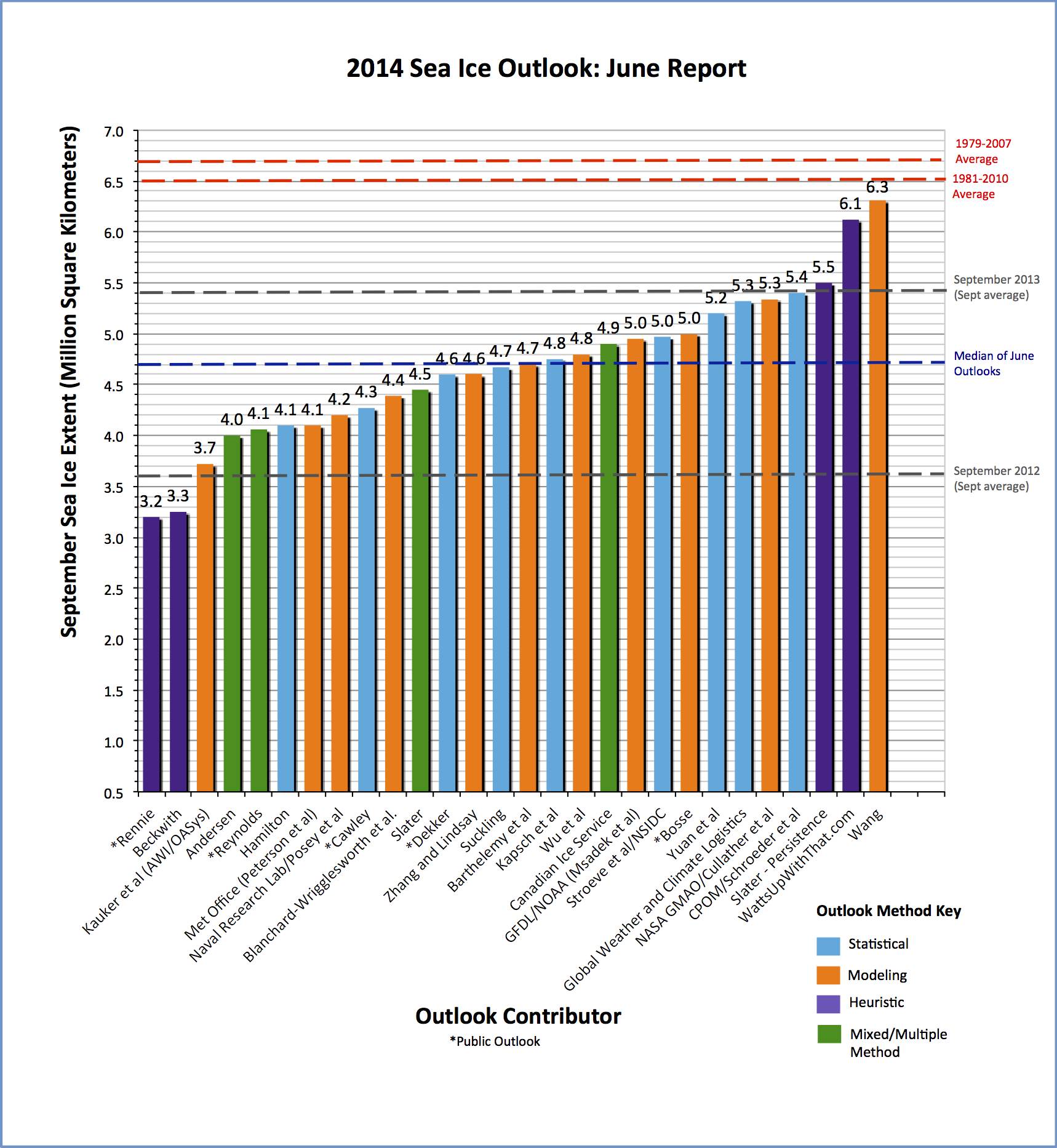
The median Outlook value for September 2014 sea ice extent is 4.7 million square kilometers with quartiles of 4.2 and 5.1 million square kilometers (See Figure 1 in the full report, below). Contributions are based on a range of methods: statistical, numerical models, estimates based on trends, and subjective information. We have a large distribution of Outlook contributions, which is not surprising given the different observed values in 2012 and 2013. The overall range is also large at 3.2 to 6.3 million square kilometers. The median outlook value is up from 4.1 million square kilometers in 2013. These values compare to observed values of 4.3 million square kilometers in 2007, 4.6 million square kilometers in 2011, 3.6 million square kilometers in 2012 and 5.4 million square kilometers in 2013. Only three outlooks this year are above the 2013 observed September extent.
As the season progresses, it will be interesting to follow the relative influences of weather (i.e., warm Arctic winter in 2013/2014 and the wind and weather through the summer) and initial conditions of the sea ice, all in the context of the long-term downward trend of sea ice extent.
This month’s full report includes the comments on modeling outlook, a summary of current conditions, key statements from each Outlook, and links to view or download the full outlook contributions. We appreciate the addition of recent ice thickness data estimated from the European Space Agency CryoSat-2 satellite, the NASA IceBridge airborne campaign, and Office of Naval Research (ONR) Marginal Ice Zone Program buoys.
See the original call for contributions for the June report here.
Full Outlook Report
Overview
Thank you to the groups that contributed to the 2014 season, 28 pan-Arctic contributions (plus one additional regional) is a record for the Sea Ice Outlook (SIO)! We appreciate the diversity of contributions. The median Outlook value for September 2014 sea ice extent is 4.7 million square kilometers with quartiles of 4.2 and 5.1 million square kilometers (See Figure 1). Thus we have a large distribution of Outlooks, which is not surprising given the different observed values from 2012 and 2013. The overall range is also large at 3.2 to 6.3 million square kilometers. The median outlook value is up from 4.1 million square kilometers in 2013. These values compare to observed values of 4.3 million square kilometers in 2007, 4.6 million square kilometers in 2011, 3.6 million square kilometers in 2012, and 5.4 million square kilometers in 2013. Only three outlooks this year are above the 2013 observed September extent. It is indeed an issue to separate the nominal downward trend in sea ice loss from year to year weather influences. Based on previous years' SIO, weather in 2007 was a factor on the low side while weather in 2013 was a factor in the high side. More sea ice at the end of summer 2013 may be offset somewhat by a warm Arctic winter in 2013/2014. We appreciate the addition of recent thickness data estimated from the European Space Agency (ESA) CryoSat-2 satellite, the NASA IceBridge airborne campaign, and Office of Naval Research (ONR) in situ buoys.
For the June report, our focus is on the pan-Arctic outlook and so there is not a separate regional report; any regional information is integrated into the full report below. We will focus on regional Outlooks in the August report, and will encourage anyone with interest in regional scale to submit their outlooks at that time.
 for September 2014 sea ice extent (values are rounded to the tenths).")
Addendum Figure, added 2 July 2014, developed by Larry Hamilton:

The Addendum Figure above shows the distribution of June 2014 Outlook contributions as a series of box plots, broken down by general type of method. The first three boxes depict contributions based on heuristic, statistical or modeling methods. For example, the median prediction of heuristically-based contributions is 4.4 million km2, compared with 4.75 for statistical and 4.7 for modeling. The fourth box or "mixed" group (median 4.5) represents contributions based on a combination of these methods, such as statistical + heuristic. Together, these first four boxes account for all 28 of the June 2014 contributions. A fifth box plot in the Addendum Figure separates out five of the modeling contributions that used both data assimilation and fully coupled modeling to arrive at their prediction. The median for this subset of the modeling group is 5 million km2. In 2013, the mean September ice extent was 5.35 million km2, indicated by a gray line across the plot. With only a handful (3 to 11) of contributions in each category, the numbers here are too small to draw analytical conclusions. We will be following these groups over the remainder of the season, however, and watching for possible patterns.
Comment On Modeling Contributions To The Sea Ice Outlook
Provided by François Massonnet, Université Catholique de Louvain
Out of 28 predictions, 10 are based on ocean–sea ice (4) or fully coupled models (6). The median predicted September sea ice extent is 4.65 million km2 (mean: 4.71 million km2). The standard deviation of individual predicted extents amounts to 0.73 million km2. All contributors provided an estimate of uncertainty around their prediction. The uncertainty was in all cases estimated using ensemble simulations. An encouraging point lies in the large number of members provided to estimate the impacts of natural variability on the prediction: on average 20 members are used per group, two groups use less than 10 members and three use more than 30. On average, the confidence intervals provided by each group (the bars in Fig. 2) have a width of 1.25 million km2. This could be interpreted as the inherent uncertainty due to the unpredictable effects of the atmosphere between June and September. Modeling groups use initial conditions obtained either from a previous run forced by atmospheric reanalyses, or initial conditions obtained directly from data assimilation of sea ice concentration or thickness.
The standard deviation between the "best estimate" predictions of all groups (the dots in Fig. 2) is 0.73 million km2, thus a +/- 2-sigma confidence interval based on all predictions would have a width of 2.92 million km2. This is larger than the contribution from natural variability (1.25 million km2, see above) and suggests that prediction uncertainty arising from structural differences (different models used, different configurations, resolutions) dominate over the uncertainty associated to natural variability.
Four groups provide maps in addition to the Pan-Arctic prediction (PDF of the four map figures). Opening of the Arctic pack near the east-Siberian coasts in September is a possibility, but the uncertainty in ice concentration in this region is large in all groups that provide this regional information. If the ice pack happens to open, the passage will probably remain tight (~500 km as estimated visually). Opening of the ice pack in the Canadian Arctic Archipelago is less likely according to these models.

Current Conditions
At the beginning of June, Arctic sea ice extent was about 400,000 square kilometers below the 1981-2010 average and slightly below the 2012 and 2013 extent on June 1 (Figure 3). However, the seasonal extent decline was generally slower than 2012 during late May and early June;the rate of decline was near-normal relative to the 1981-2010 average.
. The faded items in the key are not included on the graph. From the NSIDC Charctic Interactive Sea Ice Graph, http://nsidc.org/arcticseaicenews/charctic-interactive-sea-ice-graph/.")
The spatial pattern of loss this spring has been marked by lower than normal extent in the Barents Sea, average to above average in Baffin Bay and slightly lower than normal extent in the Bering Sea (in contrast to recent years that have had a late melt out in the Bering). By early June, a large area of open water had opened up in the Laptev Sea, substantially earlier than normal. However, within the pack, the concentration has remained high over most of the central Arctic, with some lower values developing north of Svalbard.


Arctic-average sea ice loss this spring was contributed primarily by regional loss in the seasonal ice zones of the Bering and Barents Seas due to active meteorological seasons (Figure 5). The sub-Arctic meteorology also contributed to May snow cover (see NSIDC June 3 report). The Arctic had a weak Dipole Sea Level Pressure (SLP) with a low on the Eurasian Side and a high pressure region from north of the Bering Strait across northern Canada; the SLP pattern is typical of the long term average (1981-2010). We cannot say that the spring meteorology temperature advection contributed to early melt in the central Arctic. In contrast the winter-spring temperatures over the central Arctic were higher than normal (Figure 6).

The PIOMAS sea ice volume estimates, based on a model constrained by satellite extent observations, indicate a total volume through May in line with recent years, though not at a record low (Figure 7). In general, lower early season volume suggests an average thinner overall ice cover and thus a greater potential for a lower September extent. However, May values, especially with recent years being so close together, do not provide a clear indication of potential September conditions.
Sea ice thickness estimates from the ESA CryoSat-2 altimeter (Figure 8) and the NASA IceBridge airborne campaign during March and April (Figure 9) indicate thick ice (5+ m) in the region north of Greenland and the Canadian Archipelago, but much thinner ice (~1 m) in the Beaufort and Chukchi seas, as well as the Barents and Kara seas. CryoSat-2 does show a thicker tongue of ice, ~2.5-3 m, extending from the pole to the eastern Siberian coast. This suggests that this region will be slower to melt out than surrounding areas. Airborne electromagnetic induction thickness surveys by the SIZONet project in the Chukchi and Beaufort Sea show a tongue of multiyear ice (for the first time in the past few years) extending down into this region. This suggests delayed ice retreat due to thicker ice in the region. While melt onset at Barrow was as early as it has been observed in the past 15 years with near complete snow melt in April, a cooler May and June with additional snowfall and few meltponds have pushed back complete melt of the ice cover.
Ice mass balance buoys deployed in the Beaufort Sea as part of the Office of Naval Research (ONR) Marginal Ice Zone Program indicate that surface temperatures have reached the melting point, at least intermittently, in the region, with some surface melt beginning in the southern part of the Beaufort, but little or no melt farther north (Figure 10), http://www.apl.washington.edu/project/project.php?id=miz.


, ice depth and temperature (middle) and water temperature (bottom) at Buoy Cluster 2 of the ONR Marginal Ice Zone project deployment.")
Key Statements/Executive Summaries From Individual Outlooks
The Outlooks are listed below in order of lowest to highest predicted September extent. Extent and uncertainty (in parentheses) values are provided below in units of millions of square kilometers unless noted otherwise. The individual outlooks can be downloaded as PDFs at the bottom of this webpage.
Rennie (Public), 3.20 (2.50-3.80), Heuristic
Starting with the April PIOMAS volume distribution and the April NSIDC average ice extent the estimated extent loss for each 10 cm thickness of ice loss is calculated. This calculation is then correlated with the reported 5-day average NSIDC ice extent loss. The calculation shows that the extent loss is closely correlated with the initial thickness distribution until the end of July. However the final September average figure is heavily dependent on August weather. This projection indicates a relatively slow decline in extent until mid-July, followed by a rapid decline in the last half of July, leading to a greater overall decline in extent by the end of July than occurred in 2012. In the short term the projection indicates that 2014 will not repeat the rapid decline from June 1 to 16 seen in 2012.
Beckwith, 3.25 (2.75-3.75), Heuristic
The large year-to-year variability in the sea ice extent makes this sort of prediction very dicey. Behavior of the sea ice over the past winter and the spring and the large positive temperature anomalies in the Arctic (as high as 20 degrees C over large regions in the past winter) suggest that an extent near that of the 2012 minimum may occur again if there is large export of sea ice out to the Atlantic Ocean via the Fram Strait.
Kauker et al., (AWI/OASys); 3.72 (3.30-4.14), Modeling
Estimated from ensemble coupled sea ice-ocean model runs based on atmospheric reanalyses fields from 1994-2013.
Andersen, 4.00 (3.80-4.00), Statistical/Heuristic
The estimate is based on the average years since 2007, adjusted to account for the extent peaks this past spring (short periods where the extent increased).
Reynolds (Public), 4.06 (3.49-4.63), Statistical/Heuristic
Because the decline in extent is due to increasing ease with which open water can be revealed by declining volume, a simple method is used to predict September sea ice extent based on May sea ice volume for the Arctic Ocean from the PIOMAS model.
Hamilton, 4.10 (3.10-5.10), Statistical
The 2014 extent is estimated via extrapolation of a Gompertz (asymmetric S) curve fit to the historical data.
Met Office (Peterson et al), 4.10 (3.10-5.10), Modeling
Using the Met Office GloSea5 seasonal forecast systems we have generated a model based mean September sea ice extent outlook of 4.1± 1.0 million square kilometers. This has been generated using start dates between 30 March and 19 April to generate an ensemble of 42 members.
Caveat: The ensemble mean forecast is but one of many realizations of possible September sea ice extent produced by the seasonal forecast system. Whilst the system is devised to accurately account for the range of possible outcomes, as expressed by our ensemble spread and projection uncertainty, there is still a possibility of the actual outcome falling outside this estimate.
Naval Research Lab (Posey et al), 4.20 (3.70-4.70), Modeling
The ACNFS outlook for September ice extent is 4.2 Mkm2 ± 0.5 Mkm2. The skill of the Arctic Cap model run in forward mode for a season is not yet quantified.
Cawley (Public), 4.27 (+/- 1.13), Statistical
This is essentially just a Bayesian non-parametric method used to extrapolate the trends in the observations of September sea ice in previous years, and incorporates no expert knowledge whatsoever. It is a purely statistical projection.
Blanchard-Wrigglesworth et al., 4.39 (3.89-4.89), Modeling
Our 2014 September sea ice extent forecast is 4.39 ± 0.50 million square kilometers. This is based upon a forecast using the CESM1 model initialized with sea ice anomalies obtained from the PIOMAS model for May for the period 1st May-1st October. The quoted error is obtained from the standard deviation of the ensemble distribution in September.
Our 2014 outlook calls for September sea ice to be slightly-lower than the expected linear value for 2014; in other words, lower than 2013 but unlikely (10% chance) to beat the 2012 record. We still expect it to be one of the lowest values on record. Regionally, we expect a more reduced sea ice cover in the East Siberian/Alaskan regions compared to the Atlantic facing region (Svalbard, Franz Josef)
Slater, 4.45, Statistical/Heuristic
My 50-day forecast (http://cires.colorado.edu/~aslater/SEAICE/) issued on June 6th suggests that 2014 will be near the 3rd lowest rank year on record, which is how I came to derive my estimated extent for this long-lead time. The result contains huge uncertainty and should not be considered reliable as this long-lead method has not been verified.
Dekker (Public), 4.60, (4.15-5.05 standard deviation range), Statistical
Arctic sea ice decline has global implications for Northern Hemisphere weather patterns and Arctic eco systems and wild life alike, and thus it is concerning that our global climate models so far appear to underestimate the observed rate of decline based on albedo amplification of sea ice alone.
My projection method for the decline in Arctic sea ice is based on another variable affecting how much heat the Northern Hemisphere absorbs. One that shows particularly strong correlation with Sept sea ice extent, and which I think has been underestimated in models and media articles alike: Northern Hemisphere snow cover in spring.
Zhang and Lindsay, 4.60 (4.00-5.20), Modeling
Our seasonal prediction focuses not only on the total Arctic sea ice extent, but also on sea ice thickness field and ice edge location. We feel that, for all practical and scientific reasons, it is particularly important to improve our ability to predict the ice thickness and the ice edge. Needless to say, this is a difficult goal. However, we hope that our effort would contribute to this goal.
Suckling, 4.67 (3.64-5.76), Statistical
A statistical model, known as Dynamic Climatology, is used to make the prediction for September sea ice extent in 2014. The prediction is initialised with the mean of the observed sea ice extent for September 2009-2013 and an ensemble prediction is created simply by adding all of the observed changes in the sea ice extent record from one September to the next over the historical period 1979-2013.
The ensemble members are then transformed into a probabilistic forecast distribution using the kernel dressing approach, in which the parameters of the kernels are determined based on the statistical skill over a set of hindcasts, under cross-validation.
Using this approach the mean (50th percentile) of the forecast distribution suggests a value for sea ice extent of 4.67 Million square Kilometers, with a 5-95th percentile range (3.64, 5.76) and 'likely range' (33-66%) of (4.38, 4.97).
Barthelemy et al, 4.70 (3.50-5.50), Modeling
Our estimate is based on results from ensemble runs with the global ocean-sea ice coupled model NEMO-LIM3. Each member is initialized from a reference run on May 31, 2014, then forced with the NCEP/NCAR atmospheric reanalysis from one year between 2004 to 2013. Our estimate is the ensemble median, and the given range corresponds to the lowest and highest extents in the ensemble.
Kapsch et al, 4.75 (4.13-5.37), Statistical
For the prediction of the September sea-ice extent we use a simple linear regression model that is only based on the atmospheric water vapor in spring (April/May). Thereby we assume that the spring atmospheric conditions, more precisely the greenhouse effect associated with the water vapor in the atmospheric column, are important for the seasonal prediction of the September sea-ice extent.
Wu et al, 4.80 (4.15-5.45), Modeling
The projected Arctic minimum sea ice extent from the NCEP CFSv2 model with revised CFSv2 May ICs using 31-member ensemble forecast is 4.8 million square kilometers with a SD of 0.65 million square kilometers. The maximum and minimum value for the Arctic sea ice extent from the 31-member ensemble prediction is 3.64 and 5.85 million square kilometers, respectively.
Canadian Ice Service, 4.90, Heuristic/Statistical
Three methods are combined. The first is heuristic forecast based on analyst interpretations of spring conditions. The second method uses a optimal filtering based statistical model, and the third estimate is based on regression models relating September sea ice extent to spring atmospheric and oceanic conditions.
Geophysical Fluid Dynamics Laboratory(GFDL)/NOAA (Msadek et al), 4.95 (4.24-5.55), Modeling
Our prediction for the September-averaged Arctic sea ice extent is 4.95 million square kilometers, with an uncertainty range going between 4.24 and 5.55 million square kilometers. Our estimate is based on the GFDL CM2.1 ensemble forecast system in which both the ocean and atmosphere are initialized on June 1 using a coupled data assimilation system. Our prediction is the bias-corrected ensemble mean, and the given range corresponds to the lowest and highest extents in the 10-member ensemble. Our model predicts that September 2014 Arctic sea ice extent will be 1.57 million square kilometers below the 1981 to 2010 observed average extent, but will not reach values as low as those observed in 2007 or 2012.
Stroeve et al (NSIDC), 4.97 (4.24-5.70), Statistical
We use the survival of ice of different ages to statistically predict the 2014 minimum. Summer survivability of ice age fields gives an estimate of 4.97 + 0.73 106 km2 using an average of ice survival rates from the last 5 summers (2009-2013). To estimate a range, we used estimates from the summer with the lowest (2012) and highest (2009) survival rates within the last 5 years, giving an expected range of 3.97 106 km2 to 5.82 106 km2.
Bosse (Public), 5.00 (4.55-5.45), Modeling
The approach with OHC of the year n-1 as the variable with the most important influence on the melting of the year n is a new one AFAIK. The model is plausible: The melting depends on the quantity of heat of the Arctic basin and the volume of the existing sea ice in the actual year.
Yuan et al, 5.20 (4.08-6.32), Statistical
The Markov model is capable to capture co-variability in the ocean-sea ice –atmosphere system, which is likely the predictable part of variances in sea ice. The model focuses on predicting this part of variances. Cross-validation skill, measured by correlation between four-month lead prediction and observation of September ice extent, is 0.77.
Global Weather and Climate Logistics, 5.32, Statistical
Our predictor screening approach predicts slightly more sea ice extent than last year and our anomaly correlation approach predicts slightly less sea ice extent than last year. Together the eight ensemble statistical forecasts predict 5.32 million square km of pan-Arctic sea ice extent for September 2014.
NASA Global Modeling and Assimilation Office (GMAO)/Cullather et al, 5.34 (4.90-5.78), Modeling
A projection of 5.34 ± 0.44 million km2 is made from forecasts initialized from 11 April until 1 May. The forecast has been bias corrected to NSIDC Sea Ice Index values over the previous 15-year period. This projection is made in order to understand the relative skill of the forecasting system and to determine the effects of future improvements to the system.
Centre for Polar Observation and Modelling (CPOM)/Schroeder et al, 5.40 (4.90-5.90), Statistical
We predict the September ice extent 2014 to be similar to last year. The melt-pond area in May is relatively low due to colder air temperatures and slightly thicker ice in the relevant areas of the Arctic in comparison to the last 5 years.
Slater ("Persistence" Outlook), 5.50 [average of three values], Heuristic
Three different types of persistence forecasting at long lead-time were used. The three values were then averaged. The methods contain no skill.
WattsUpWithThat.com, 6.12, Heuristic
A poll was conducted on June 10th, 2014 (http://wp.me/p7y4l-sVu ) of readers of wattsupwiththat.com regarding the Sept. Average Sea Ice extent. 519 votes were cast with a selection of values ranging from 8 million to 3 million square kilometers. Predictions were supplemented by NCEP/NOAA's new CFSv2 model that showing an above-normal ice extent for Sept, 2014, seen here:
https://wattsupwiththat.files.wordpress.com/2014/06/cfsv2_capture_june1….
Wang, 6.31 (5.84-6.78), Modeling
The projected Arctic sea ice extent from CPC based on NCEP ensemble mean CFSv2 forecast is 6.31×10⁶ km2 with an estimated error of ±0.47×10⁶ km2.
Additional Regional Outlook
Gudmandsen, Nares Strait Region, Heuristic
A heuristic forecast for the timing of break-up for the ice arch in Kennedy Channel is the beginning of July. The forecast is based on early June temperatures (-3° C) and the formation of narrow leads that normally precede break-up. A large floe in Robeson Channel is also blocking the flow of multi-year ice through Nares Strait. The timing of melt/break-up of this floe is hard to predict.
Individual Outlook PDFs
| Attachment | Size |
|---|---|
| Anderson35.96 KB | 35.96 KB |
| Barthelemy et al.326.93 KB | 326.93 KB |
| Beckwith46.2 KB | 46.2 KB |
| Blanchard-Wrigglesworth et al.592.52 KB | 592.52 KB |
| Bosse77.04 KB | 77.04 KB |
| Canadian Ice Service922.93 KB | 922.93 KB |
| Cawley58.56 KB | 58.56 KB |
| CPOM Schroeder et al.47.32 KB | 47.32 KB |
| Dekker29.07 KB | 29.07 KB |
| GFDL NOAA Msadek et al.198.48 KB | 198.48 KB |
| Global Weather Climate Logistics215.87 KB | 215.87 KB |
| Gudmandsen428.82 KB | 428.82 KB |
| Hamilton267.97 KB | 267.97 KB |
| Kapsch et al.57.57 KB | 57.57 KB |
| Kauker et al.178.13 KB | 178.13 KB |
| Peterson et al.133.29 KB | 133.29 KB |
| NASA GMAO Cullather et al.2.56 MB | 2.56 MB |
| NRL Posey et al.502.48 KB | 502.48 KB |
| Rennie182.08 KB | 182.08 KB |
| Reynolds247.23 KB | 247.23 KB |
| Slater54.25 KB | 54.25 KB |
| Slater Persistence101.53 KB | 101.53 KB |
| Stroeve et al.627.78 KB | 627.78 KB |
| Suckling107.2 KB | 107.2 KB |
| Wang64.79 KB | 64.79 KB |
| WUWT24.59 KB | 24.59 KB |
| Wu et al.156.58 KB | 156.58 KB |
| Yuan et al.55.54 KB | 55.54 KB |
| Zhang and Lindsay246.3 KB | 246.3 KB |
 for September 2014 sea ice extent (values are rounded to the tenths).")