
Pan-Arctic Summary
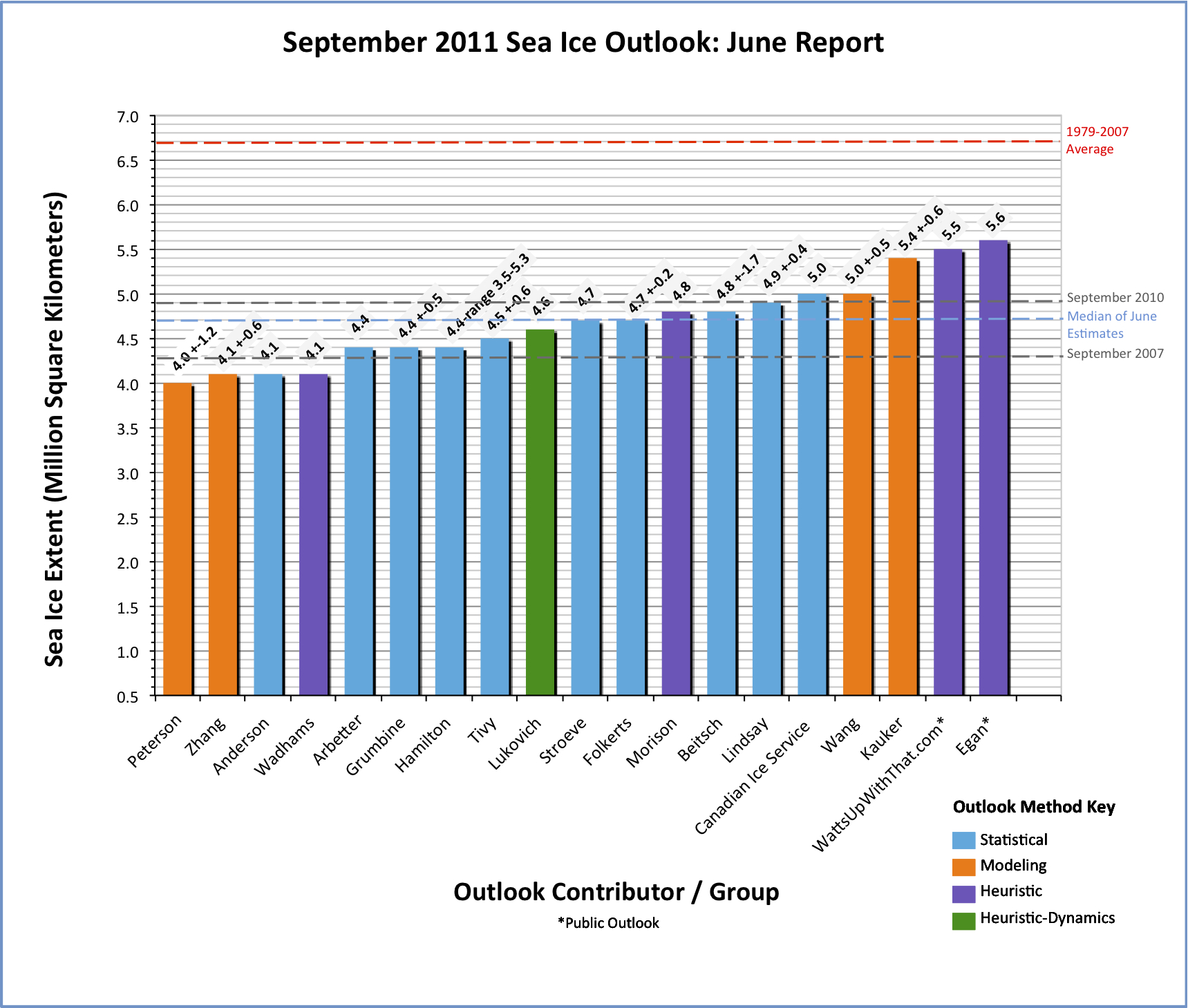
The 2011 June Outlook suggests a modest decrease for summer 2011. With 19 responses for the pan-arctic (and 7 for the regional outlook), including several new contributors, the June Sea Ice Outlook projects a September 2011 arctic sea extent median value of 4.7 million square kilometers (Figure 1). This compares to observed September values of 4.7 in 2008, 5.4 in 2009, and 4.9 in 2010. The range of values is 4.0 to 5.6 million square kilometers, but the distribution is skewed toward lower values, suggesting either persistent conditions or a substantial drop below 2008 and 2010 values and the long-term downward trend. The 2011 June Outlook differs from the 2010 Outlook by not including projections of major increases in extent. It is important to note for context that all 2011 estimates are well below the 1979–2007 September climatological mean of 6.7 million square kilometers.
Individual responses were based on a range of methods: statistical, numerical models, comparison with previous observations and rates of ice loss, and composites of several approaches. The consensus of a stable low level of sea ice extent or continued modest sea ice loss is a strong result. The range of Outlook values suggest that most uncertainty lies in the separate methods to the Outlook.
 for September 2011 sea ice extent.")
Download High Resolution Version of Figure 1.
Credit for Sea Ice Outlook Report: Arctic Research Consortium of the US (ARCUS)
Pan-Arctic Full Outlook
OVERVIEW OF RESULTS
With 19 responses, including several new contributors (thank you), the June Sea Ice Outlook projects a September 2011 arctic sea extent median value of 4.7 million square kilometers with quartiles of 4.4 and 4.95 million square kilometers (Figure 1). This compares to observed September values of 4.7 in 2008, 5.4 in 2009, and 4.9 in 2010. The distribution of the June Outlooks is skewed toward lower values, with a range of 4.0 to 5.6 million square kilometers, suggesting either persistent conditions or a substantial drop below 2008 and 2010 values and the long-term downward trend. The 2011 June Outlook differs from the 2010 Outlook by not including projections of major increases in extent. It is important to note for context that all 2011 estimates are well below the 1979–2007 September climatological mean of 6.7 million square kilometers.
Individual responses were based on a range of methods: statistical, numerical models, comparison with previous observations and rates of ice loss, composites of several approaches, or 'educated guesses' based on various datasets and trends (included in the heuristic method category). The median of individual uncertainty estimates, where provided, is ±0.6 million square kilometers (near the values suggested from last year), with quartiles of ±0.5 and ±0.9. Similar to the 2010 Outlook, the range of the four numerical modeling methods represents examples of both persistence and low Outlook values. The range of all Outlook values and the range of Outlook values within method categories are larger than implied by individual uncertainty estimates, suggesting most uncertainty lies in the separate approaches to the Outlook. Still, the consensus of a stable low level of sea ice extent or continued modest sea ice loss is a strong result.
Outlooks are not firm forecasts, but promote a discussion of the physics and factors of summer sea ice loss. Again in 2011, we are pleased at the extent of methods and discussion and thank the contributors for their efforts.
Download High Resolution Version of Figure 1.
As discussed in the section below on late spring 2011 conditions, May 2011 looked similar in many respects to May 2010 and supports an early sea ice loss. Total sea ice extent for the previous three months was near or below the level of 2007, the year with the lowest minimum summer ice extent during the satellite record. Ice-free areas were beginning to open up in the northern Kara Sea and north of Bering Strait. There were arctic-wide positive temperature anomalies with hot spots in recently open water areas. The Arctic Dipole (AD) climate pattern, which advects heat and moisture across the western Arctic from the south, is present. However, the Climate Prediction Center's 8- to 14-day atmospheric forecast suggests a weakening of the AD during June.
This brings up one of the most important questions in arctic science. The September sea ice extent for every year since 2007 has been lower than all extents prior to 2007 (Figure 2) and there is no reason to expect 2011 to be wildly different. Does this suggest a new level of reduced summer ice extent persisting at around 5.0 million square kilometers, relative to a value of 6.0 million square kilometers in the early 2000s? If so, what is driving this transition and when will summer sea ice extent drop down to a lower level? Climate models suggest periods of stability (with variations around a stationary summer mean extent) with intermittent years of rapid reductions in ice extent as the Arctic warms (see Serreze, Mark C. 2011. Climate change: Rethinking the sea-ice tipping point. Nature 471, 47–48, doi:10.1038/471047a). Perhaps the ice extent in summer is conditioned by the rapid growth rate and thickness of the newly expansive regions of first-year sea ice? Are these regions of first-year sea ice vulnerable to early melt? Or will it take additional arctic warming to increase the probability for the next major drop in summer sea ice extent? The contributors to the 2011 Outlook suggest a modest decrease for summer 2011.

LATE SPRING 2011 CONDITIONS
Regarding initial conditions for Spring 2011, Figure 3 by Jim Maslanik and others shows maps of sea ice classes derived from sea-ice age for the end of January and May 2011. Their approach to determining sea-ice age is based on tracking of sea ice using satellite imagery. Purple regions are areas of first-year sea ice. An interesting feature in both images is the tongue of old sea ice (white) extending into the southern Beaufort Sea. According to Maslanik, "the reduced extent apparent at the end of May compared to January reflects transport associated with a mostly positive Arctic Oscillation situation in winter, followed by negative Arctic Dipole (positive dipole anomaly) in April and May. Please keep in mind that these maps basically indicate areas where at least some multiyear (MY) ice is expected to be present rather than areas where MY ice is prevalent." (personal communication). The ice age plot is supported by several ice thickness flights carried out by the Alfred Wegener Institute in collaboration with University of Alberta and University of Alaska Fairbanks in this region, which found a thinner mode of total level first-year ice thickness north of Barrow (1.4 m compared to 1.7-1.9 m in previous years) and little, comparatively thin multiyear ice in regions showing old ice in Maslanik's data. Pending further analysis, there are indications that this situation—presence of some MY ice mixed in with substantial amounts of first-year ice—is increasingly common. This also helps explain differences in ice type distributions obtained from radar- and passive microwave-derived MY ice extents.

Figure 4 shows a loss of sea ice extent through May below the 2007 level (National Snow and Ice Data Center plot); contributions to the loss were especially important from the Barents and Chukchi Seas (Figure 5). Similar to 2010, such loss can be related to warm temperatures throughout the Arctic during May (Figure 6). Given the hint of a sea ice-free region near the New Siberian Islands (off the Siberian Coast) in Figure 5 and the temperature maximum in Figure 6, one might suggest an early sea-ice melt along the Siberian coast this summer. The North Atlantic Oscillation turned positive in spring and can be seen as low sea level pressures over Iceland during May 2011 (Figure 7). Compared to positive temperature anomalies over southern Baffin Bay as in 2010, temperature anomalies are now negative. Stroeve has pointed out that we had an Arctic Dipole (AD) pattern in May 2011 with geostrophic flow directed across the top of the Arctic (Figure 7); this contrasts with May climatology, which has high pressure over the central Arctic and weak gradients. However, the AD pattern may be weakening in June, according to the Climate Prediction Center's 8- to 14-day forecast. Overall, the curve shown in Figure 4 is commensurate with the notion that a thinner arctic ice cover that is more mobile in May 2011 can lead to continuing relative sea ice loss.
.")
.")


KEY STATEMENTS FROM INDIVIDUAL OUTLOOKS
Key statements from the individual Outlook contributions are below, summarized here by author, organization of first author, Outlook value, standard deviation/error estimate (if provided), method, and abstracted statement. The statements are ordered from highest to lowest outlook values. Each individual contribution is available in the "Pan-Arctic Individual PDFs" section at the bottom of this webpage. We should have another interesting season this year; stay tuned for next month's Outlook in July!
Egan (public contribution); 5.6; Heuristic
Reason: eyeballing current shape in 2011 - looks like 2005.
WattsUpWithThat.com (public contribution-poll); 5.5; Heuristic
Website devoted to climate and weather polled its readers for estimates of the 2011 sea ice extent minimum by choosing bracketed values from a web poll, which can be seen at: http://wattsupwiththat.com/2011/05/19/sea-ice-news-call-for-arctic-sea-…
Kauker et al. (Alfred Wegener Institute for Polar and Marine Research); 5.4 ± 0.6; Model
For the present outlook the coupled ice-ocean model NAOSIM has been forced with atmospheric surface data from January 1948 to 18 May 2011. This atmospheric forcing has been taken from the NCEP/NCAR reanalysis (Kalnay et al., 1996). We used atmospheric data from the years 1991 to 2010 for the ensemble prediction. The model experiments all start from the same initial conditions on 18 May 2011. We thus obtain 20 different realizations of sea ice development in summer 2011. Since the forward simulation underestimates the September extent compared with the observed extent minima in 2007, 2008, and 2009 by about 0.49 million km2 (in the mean), we added this bias to the results of the ensemble. It is not clear whether the bias is caused by an imperfect sea ice-ocean model or by imperfect initial or boundary conditions.
Wang et al. (NOAA/NWS/NCEP); 5.0 ± 0.5; Model
The outlook is based on a CFSv2 ensemble of 40 members initialized from 17-26 May 2011. The model's systematic bias has been removed based on its retrospective forecasts for 1982-2010.
Canadian Ice Service; 5.0; Statistical
As with Canadian Ice Service (CIS) contributions in June 2009 and June 2010, the 2011 forecast was derived using a combination of three methods: 1) a qualitative heuristic method based on observed end-of-winter Arctic Multi-Year Ice (MYI) extents, as well as an examination of Surface Air Temperature (SAT), Sea Level Pressure (SLP) and vector wind anomaly patterns and trends; 2) an experimental Optimal Filtering Based (OFB) Model which uses an optimal linear data filter to extrapolate NSIDC's September Arctic Ice Extent time series into the future; and 3) an experimental Multiple Linear Regression (MLR) prediction system that tests ocean, atmosphere, and sea ice predictors.
Lindsay and Zhang (Applied Physics Laboratory, U. of Washington); 4.9 ± 0.4; Statistical
Our statistical prediction is made with PIOMAS model data from the average of May 2011. We are using May data for the 23 years 1988 through 2010 to fit the regression model and then the ice conditions for 2011 to make the predictions. The best single predictor is the fraction of the area with open water or ice less than 1.0 m thick, G1.0. This predictor explains 77% of the variance.
Beitsch et al. (University of Hamburg); 4.8 ± 1.7; Statistical
The KlimaCampus's outlook is based on statistical analysis of satellite derived sea ice area. We introduced following improvements: high resolution (AMSR-E) sea ice concentration data, a time-domain filter that reduces observational noise, and a space-domain selection that neglects the outer seasonal ice zones. Thus, small scale sea ice openings like coastal polynyas that might inhere some predictive capability for the sea ice minimum can be better utilized. The daily estimate of the September extent, the anomaly of the current day and the time series of daily estimates since May 2011 can be found on our ftp server: ftp://ftp-projects.zmaw.de/seaice/prediction/
Morison and Untersteiner (Polar Science Center, APL-UW); 4.8; Heuristic
So far this year, ice conditions seem to be similar to last year, and indeed considering the Northern Sea Ice Anomaly plot from David Chapman's Cryosphere today Website, the annual cycles of extent since 2008 have been similar. The ice in the central Arctic Ocean in April during this years North Pole Environmental Survey (NPEO) deployment was again dominantly first year ice, but seemed more deformed than usual suggesting greater average thickness, a positive factor in extent. The winter 2010-2011 Arctic Oscillation was negative at least initially, a positive factor for ice extent in September, but over the whole winter not as negative as 2010.
Folkerts (Barton Community College); 4.7 ± 0.2; Statistical
Estimates are based on multiple regression of a wide variety of publicly available monthly arctic data (e.g., extent, area, sea surface temperature, North Atlantic Oscillation, and so forth). Data from 5 to 18 months before September (i.e., from March of the previous year thru April of the given year, but not from May) were correlated with the September monthly average extent data during the period 1979-2010.
Stroeve et al. (National Snow and Ice Data Center); 4.7; Statistical
NSIDC is using the same approach as last year: survival of ice of different ages based on ice age fields provided by Chuck Fowler and Jim Maslanik (Univ. Colorado, Boulder). However, this year we are using a revised ice age product, one based on a 15% sea ice concentration threshold rather than the earlier version, which used a threshold of 40% (see Maslanik et al., in review for more details).
Lukovich et al. (Centre for Earth Observation Science, U. of Manitoba); 4.6; Heuristic-Dynamics
Investigation of dynamical atmospheric contributions in spring to sea ice conditions in fall, based on comparison of 2011 and 2007 stratospheric and surface winds and sea level pressure (SLP) in April and May suggests regional differences in sea ice extent in fall, in a manner consistent with recent studies highlighting the importance of coastal geometry in seasonal interpretations of sea ice cover (Eisenman, 2010). The absence of anomalous features evident in 2007 in SLP and stratospheric and surface winds in spring in 2011 indicates that accelerated decline associated with the former will not be an artifact of dynamical phenomena, although a thinner and more mobile ice cover may lower the wind forcing threshold required for increased ice export. Lower ice concentrations in 2011 relative to 2007 in late May indicate increased sensitivity of the arctic ice cover to atmospheric dynamical forcing, with implications for ice transport during summer.
Tivy (University of Alaska Fairbanks); 4.5 ± 0.6; Statistical
Statistical - canonical correlation analysis (CCA). A persistence forecast based on February ice concentration anomalies is generated using CCA. February is chosen over May because the correlation with September extent is higher. The model is trained on the 1980-2010 period using the passive microwave derived data set (nasateam).
Hamilton (University of New Hampshire); 4.4, range 3.5 to 5.3; Statistical
This is a naive, purely statistical model. It predicts September mean extent simply from a Gompertz curve representing the trend over previous years. Estimation data are
NSIDC monthly mean extent reports from September 1979 through September 2010.
Grumbine et al. (NOAA/NWS/NCEP); 4.4 ± 0.5; Statistical
The physical basis of the statistical method is to model the growth of open water as a feedback process analogous to population growth under constraint. This produces a logistic curve. The statistics are used to estimate the three parameters for such curves.
Arbetter et al. (National Ice Center); 4.4; Statistical
The system determines the relationships between sea ice and atmospheric conditions over the past ten years to determine the likelihood of ice being present this year. The model uses SSM/I sea ice concentration, NCEP 2m Air Temperature, and NCEP Sea Level Pressure, and correlates each point with every other point in the domain, in a brute force multiple linear regression.
Wadhams (University of Cambridge); 4.1; Heuristic
Based on recent EM measurements of first year ice thickness merged into probability density functions of ice thickness from recent submarine voyage and subtracting an assumed summer melt of up to 2 m.
Anderson (Norwegian Space Centre); 4.1; Statistical
We have looked into the yearly change of the sea ice area. This would be a first order indication of the fraction of ice that melts. Since it is the area that is measured this does not account the variation of sea ice thickness, which is needed to understand the total melt. All the data used are taken from http://arctic-roos.org/. The simplest way to look at this is to take the difference between the maximum winter sea ice area (Aw) and compare it with the minimum area (As) the following summer season. Fig. 1 [see PDF of contribution in section below] shows the value (Aw –As) /Aw from 1979-2010.
Zhang (Applied Physics Lab, University of Washington); 4.1 ± 0.6; Model
This is based on numerical ensemble predictions starting on 6/1/2011 using the Pan-arctic Ice-Ocean Modeling and Assimilation System (PIOMAS). The ensemble consists of seven members each of which uses a unique set of NCEP/NCAR atmospheric forcing fields from recent years, representing recent climate, such that ensemble member 1 uses 2004 NCEP/NCAR forcing, member 2 uses 2005 forcing, and member 7 uses 2010 forcing.
Peterson et al. (UK Met Office); 4.0 ± 1.2; Model
This projection is an experimental prediction from the UK Met Office seasonal forecast system, GloSea4 (Arribas et al., 2011). GloSea4 is an ensemble prediction system using the HadGEM3 coupled climate model (Hewitt et al., 2011). A further bias toward lower ice thicknesses in the actual forecast as compared to the hindcast initialization is also suspected. Therefore, we suspect that our forecast may be biased towards a smaller ice extent from the ultimate reality. Furthermore, this bias appears to become even more exaggerated with later start dates, hindering our ability to update the forecast at a later time.
Update provided after report was published: Wu, Grumbine, Wang (provided 6/24)
Estimate: 4.8 million square km with standard error of 0.2 million square km
Basis: We ran the CFS with 20 December 2010 initial conditions and 10 Initial conditions from January 2011. These were modified from the CFS v2.0 initial conditions by thinning the ice pack by 60 cm -- the thickness which we used as a cutoff in making our 2010 SIO estimates. If this thinning would have eliminated ice from areas observed to have sea ice, a minimum thickness of 20 cm was left in place. In making our estimate for September 2011, directly using the model's extent again seemed excessive (see also Wang's estimate). But the initial condition change does appear to have improved the model's behavior, and a critical thickness of 30 cm was used this year against last year's 60 cm.
| Attachment | Size |
|---|---|
| Andersen151.39 KB | 151.39 KB |
| Arbetter et al.301.07 KB | 301.07 KB |
| Beitsch et al.3.14 MB | 3.14 MB |
| Egan17.82 KB | 17.82 KB |
| Folkerts35.77 KB | 35.77 KB |
| Grumbine et al.32.79 KB | 32.79 KB |
| Hamilton170.13 KB | 170.13 KB |
| Kauker et al.235.45 KB | 235.45 KB |
| Lindsay and Zhang277.9 KB | 277.9 KB |
| Lukovich et al.515.72 KB | 515.72 KB |
| Morison and Untersteiner28.03 KB | 28.03 KB |
| Peterson et al.1.23 MB | 1.23 MB |
| Stroeve et al.194.19 KB | 194.19 KB |
| Tivy97.53 KB | 97.53 KB |
| Wadhams32.65 KB | 32.65 KB |
| Wang et al.133.11 KB | 133.11 KB |
| Watts and Poll43.5 KB | 43.5 KB |
| Wohlleben659.67 KB | 659.67 KB |
| Zhang247.59 KB | 247.59 KB |
| Wu et al. (contribution provided after report released)30.59 KB | 30.59 KB |
| Peterson et al. (revised contribution after report released)1.24 MB | 1.24 MB |
| Attachment | Size |
|---|---|
| Gerland et al.1.07 MB | 1.07 MB |
| Gudmandsen504.38 KB | 504.38 KB |
| Howell730.47 KB | 730.47 KB |
| Lindsay and Zhang358.32 KB | 358.32 KB |
| Petrich et al.702.17 KB | 702.17 KB |
| Tivy703.68 KB | 703.68 KB |
| Zhang247.59 KB | 247.59 KB |
 for September 2011 sea ice extent.")