
Sea Ice Outlook 2015: DRAFT Post-Season Report
DRAFT POST-SEASON REPORT
Request for Input
The 2015 Sea Ice Outlook (SIO) Action Team invites community comment on its draft post-season report. This draft includes the main post-season analysis and discussion points, although some parts are still under development and editing.
The SIO Action Team aims to have a final draft ready to share with the larger community during the 2015 American Geophysical Fall Meetings 14-19 December. Your comments on the analysis and discussion sections as well as suggestions on how to help improve sea ice forecasts are welcome.
The report found below is also available for download below as a PDF or as a Microsoft Word document. Comments may be sent as text via email or by using the "Track Changes" tool in Microsoft Word.
Please send your comments to Betsy Turner-Bogren (betsy [at] arcus.org) no later than Friday, 11 December 2015.
On behalf of the 2015 SIO Action Team, thank you for your input.
![]() 2015 Draft Post Season Report (PDF - 4.2 MB)
2015 Draft Post Season Report (PDF - 4.2 MB)
![]() 2015 Draft Post Season Report (DOCX - 5.2 MB)
2015 Draft Post Season Report (DOCX - 5.2 MB)
HIGHLIGHTS and TAKE-HOME POINTS
- The September 2015 Arctic sea ice extent was the fourth lowest extent observed in the modern satellite record, which started in 1979, at 4.63 million square kilometers according to National Snow and Ice Data Center (NSIDC) estimates.
- Following the relatively cool May and June, the Arctic experienced one of the warmest Julys on record, which led to rapid ice loss through the month.
- This year we had a total of 105 submissions from June through August focused on pan-Arctic conditions and a total of three regional submissions.
- New content in this report includes an extended analysis and discussion of the modeling contributions.
Introduction
We appreciate the contributions by all participants and reviewers in the 2015 Sea Ice Prediction Network (SIPN) Sea Ice Outlook (SIO). The SIO, a contribution to the Study of Environmental Arctic Change (SEARCH), provides a forum for researchers to contribute their understanding of the state and evolution of Arctic sea ice, with a focus on forecasts of the Arctic summer sea ice minima, to the wider Arctic community. The SIO is not a formal forecast, nor is it intended as a replacement for existing forecasting efforts or centers with operational responsibility. Additional background material about the Outlook effort can be found on the background page. With funding support provided by a number of different agencies, the SIPN project provides additional resources and a forum for discussion and synthesis. This year we received a total of 105 submissions from June to August, with 31 individual submissions focused on pan-Arctic conditions for June, 34 for July, and 37 for August. We also had one regional submission in June, one in July, and one in August.
Pan-Arctic Overview
The September 2015 Arctic sea ice extent was 4.63 million square kilometers, based on the processing of passive microwave satellite data using the NASA Team algorithm, as used by the National Snow and Ice Data Center (NSIDC). This is the fourth lowest September ice extent observed in the modern satellite record, which started in 1979 (Figure 1). It is 1.87 million square kilometers lower than the 30-year average for 1981-2010 and 1.01 million square kilometers greater than the current record low September ice extent observed in 2012 (see Figure 1).
. Least-square linear trend line is shown blue.")
While the SIO uses the monthly NSIDC sea ice extent estimate (based on the NASA Team algorithm) as its primary reference, there are several additional algorithms that have been developed over the years to derive sea ice concentration and extent from passive microwave sensors. These various algorithms employ different methodologies and combinations of microwave frequencies and polarizations. While no single algorithm has been found to be clearly superior in all situations, the algorithms show differences in their sensitivity to various ice characteristics (ice thickness, snow cover, surface melt) and the surrounding environment (the atmosphere), resulting in differences in the estimated ice concentration and extent. In addition, the algorithms may use different source data and employ different processing and quality-control methods. The different source data is particularly important. Products from the JAXA AMSR2 sensor have higher spatial resolution than those using the DMSP SSMIS sensor, and thus have a great potential precision in locating the ice edge.
The range of the algorithms provides an indication of uncertainty in the observed extent. To augment the NSIDC value, we provide estimates from selected other algorithms that are readily available on-line (thanks to G. Heygster, Univ. Bremen, for providing Bremen ASI values; and J. Comiso and R. Gersten, NASA Goddard, for providing Bootstrap values).
The trajectories of daily ice extent estimated using various ice concentration datasets are shown in Figure 2. This highlights the variation in ice extent and the estimated date of the summer minimum found across these different observational products. All but NERSC's Arctic-ROOS algorithm are generally within ~400,000 square kilometers and the range of monthly and daily extent after removing the highest and lowest outliers is 310,000 and 290,000 square kilometers respectively (Table 1).
 for 1 June – 30 September 2015. A 5-day running average is applied to the daily values.")
| Product | Sep Avg | Min Daily | Source Website |
|---|---|---|---|
| NSIDC SII* | 4.63 | 4.41 | http://nsidc.org/data/seaice_index/ |
| NSIDC NT | 4.57 | 4.41 | http://nsidc.org/data/seaice_index/ |
| GSFC BT | 4.88 | 4.68 | http://neptune.gsfc.nasa.gov/csb/ |
| JAXA BT | 4.47 | 4.31 | https://ads.nipr.ac.jp/vishop/vishop-extent.html?N |
| NERSC Norsex Arctic-ROOS | 5.47 | 5.25 | http://arctic-roos.org/observations/ |
| Bremen | 4.63 | 4.48 | http://www.iup.uni-bremen.de:8084/amsr2/ |
| MASIE | 4.66 | 4.48 | http://nsidc.org/data/masie/ |
| Avg (all) | 4.75 | 4.57 | |
| Avg (-outliers) | 4.67 | 4.49 | |
| Range (-outliers) | 0.31 | 0.29 |
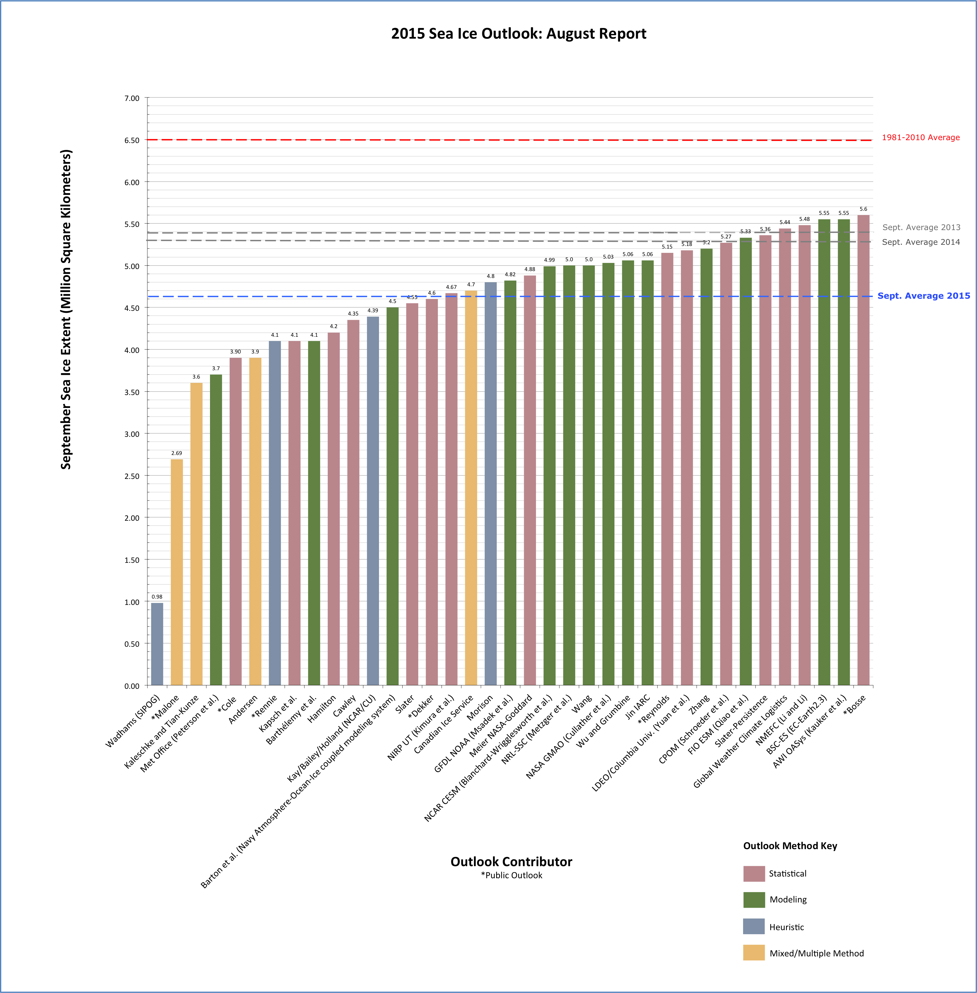
There were 37 pan-Arctic Outlook contributions in August, covering a range of different methodologies: (1) statistical methods that rely on historical relationships between extent and other physical parameters, (2) dynamical models, (3) and heuristic methods such as naïve predictions based on trends or other subjective information. The median August estimate was 4.8 million square kilometers, with a quartile range of 4.2 to 5.2 million square kilometers (Figure 3). This was a small downward adjustment from June and July (5.0, quartile range: 4.4-5.2) and represents an improved estimate relative to the observed extent as the forecast period shortened and information from June and July could be incorporated. However, we note that many contributions did not adjust their estimates for June and/or July.
 for September 2015 extent.")
Download a high-resolution version of Figure 3.
The median Outlooks performed reasonable well relative to standard baseline metrics of persistence (i.e., use 2014 value to estimate 2015) and trend (extrapolate the 1979-2014 trend line to estimate 2015). The median of 4.8 million square kilometers was significantly lower than the persistence value of 5.28 million square kilometers, but was roughly the same as the extrapolated trend estimate of 4.76 million square kilometers. As noted in Stroeve et al. (2014), the Outlook predictions tend to better match the observations when the observed extent is near the trend line (Figure 4). Thus the good performance this year does not necessarily indicate an improvement in skill but rather an easier year to predict as it coincides with the forced trend.
 and negative (2007 and 2012, blue) departures are highlighted.")
Splitting the contributions by method indicates little changes in predictions over the three months (again, many contributions did not update their analysis from June) (Figure 5). The heuristic and statistical methods did converge toward the final observed value in August, while the models changed only a small amount and the contributions from the mixed methods actually diverged from the September value. The small model change may be due to most models not being reinitialized and resubmitting June estimates. The poor performance of the mixed method may be simply due to the low number of submissions (only 10 total over the three months).

The continual evolution of forecasting systems and incomplete submission for all lead times means that generalizations are difficult to make. There is substantial error variance within each of the above-mentioned Outlook groups perhaps because the differences in the details of techniques within each group can be considerable. However, some individual forecasts/projections tend to be more consistent than others, at least within the past few years (when the number of contributions has increased; see Figure 6 below). While the top four performers in August 2015 were statistical methods, if we look at performance over time, the four best modeling efforts would have provided better performance than the four top statistical methods. Note also that the top five performers in Figure 6 are based on spatially explicit information rather than prediction of a single extent number. However, as has been stated our analysis is incomplete and limited by the format of the SIO. A more systematic approach to forecasting evaluation, using reproducible methods, is needed if we are to advance.

Review of Arctic 2015 Summer Conditions
The summer sea ice retreat began earlier than normal with the maximum (winter) extent occurring about two weeks early on 25 February. (See: NSIDC Arctic Sea Ice News & Analysis, 19 March 2015.) It was also the lowest maximum extent in the satellite record. However, the melt season overall got off to a relatively slow start. May and June temperatures were near or below average (Figure 7) and extent declined at average or even below average rates through the end of June. In particular, melt started later than normal in Baffin Bay and ice lingered longer than usual into the summer. However, in some regions warm conditions were experienced. For example, Barrow, Alaska experienced its warmest May on record and snow disappeared by May 28, the second earliest date since records began 73 years ago. This led to surface melt beginning a month earlier than normal in the southern Beaufort Sea. The Kara Sea also experienced early melt onset. Sea ice in both the Beaufort and Kara regions opened up relatively early. (See: NSIDC Arctic Sea Ice News & Analysis, 5 August 2015.)
Following the relatively cool May and June, the Arctic experienced one of the warmest Julys on record, which led to rapid ice loss through the month. The warm July was likely related to higher than normal sea level pressure over the central Arctic during the month (Figure 8), which indicates relatively clearer skies (and more incoming solar radiation). The high pressure over the Arctic was accompanied by lower pressure over northern Eurasia. This pattern helps funnel warm air into the Arctic from the south and compact sea ice into a smaller area. A very similar pattern characterized much of the 2007 summer. The rapid ice loss continued well into August and for a brief time, it appeared that 2015 might surpass 2012. However, extent loss slowed considerably in late August and into September.
 to warmest (red). The 2015 ranking for each month is in yellow.")

The year began with considerable multi-year ice in the Beaufort and Chukchi seas, as indicated by sea ice age data. (See: NSIDC Arctic Sea Ice News & Analysis, 6 October 2015. However, much of the older ice in this region melted over the summer, similar to many summers over the past decade.
Regional Contributions
Four groups submitted regional contributions of sea ice extent probability (SIP) for the June outlook (NASA, NRL, UCL and MetOffice), two groups for the July outlook (NCAR, NRL), and three groups for the August outlook (Slater, NRL and MetOffice). All models apart from Slater are dynamical models, whereas Slater is a statistical model. Below in Figure 9 we show the forecasted SIPs with the observed September 2015 sea ice edge and in Figure 10 the Brier scores from each forecast and the multi-model mean. We also show the SIP and Brier score from a statistical forecast obtained by extending the 1979-2014 linear trend at each grid point.
In both plots, we break down the forecast submissions into the earliest (June call) and latest (August call) forecasts. From visual inspection of Figure 9, an improvement in August forecast SIPs relative to June forecast SIPs can be discerned. The model-mean June SIP forecast shows very high (low) SIPs in the Beaufort Sea (Laptev/Kara), which are partly corrected in the model-mean August SIP forecast. The improvement in the model-mean August SIP forecast is confirmed by the Brier scores in Figure 10 (lower Brier scores represent a more accurate forecast). Another interesting result is that the multi-model mean forecast for each call is more accurate than all individual model forecasts for the same call. As in 2014, the August statistical forecast of Slater shows a high degree of skill. We also produce a statistical linear forecast of SIP by taking the sea ice extent at each grid cell (1 for sea ice concentration > 0.15, 0 for sea ice concentration < 0.15), fitting a line of best fit over 1979-2014 and extrapolating the fit to 2015. This forecast shows very good skill, which is not too surprising considering that the total 2015 extent was very close to the linear fit (see Figure 1 above).
 for the 4 models from June call, 3 models from August call, model means, and linear forecast SIP. The black contours in the panels indicate the September 2015 sea ice edge, while the month labels indicate initialization times for the different models.")
 forecast. The numbers on the x-label of each panel show the Arctic-wide mean Brier score, which is averaged over the Arctic basin, while the month labels indicate initialization times for the different models.")
We also received forecasts of Ice Free Dates (IFDs) from NRL and NASA GMAO. Below we show the IFDs from the June call (Figure 11). While there are biases in the model forecasts, late IFDs (or even perennial ice) are forecast in the Beaufort and East Siberian seas, and early IFDs are forecast in the Laptev and Kara seas. In this region, the NRL forecast does remarkably well. In Baffin Bay, models forecast an earlier melt than observed.
 forecasts from NRL and NASA GMAO from the June SIO call.")
Summary of Modeling Contributions
There were 14 contributions from modeling groups for the August Outlook, some of them being simply duplicates of the July or June submissions. Nine submissions were done using fully-coupled atmosphere-ocean-(land)-sea ice models and five using ocean-sea ice models forced by atmospheric reanalysis of previous years or output from an atmospheric model.
In the 2014 SIO Post-Season Report we discussed the evolution over time (from June to August) of the model predictions and found that this ensemble was becoming more certain (collectively and for models individually) as the initialization date approached September. This pattern is less clear this year (Figure 5 and Figure 12), suggesting either that predictability associated to initial conditions was less important in 2015 than last year, or that sampling errors are large due to the small ensemble size. Either way, we note that only six groups provided three distinct outlooks for June, July and August, making it difficult to discern common patterns.
 and green (ocean-sea ice). Values for June and July are shown in lighter colors. The dots are the outlook estimates themselves and the intervals are the uncertainty ranges provided by the groups. Definitions of uncertainty were left to the discretion of the groups themselves, and should therefore be compared with caution. The middle dashed horizontal line is the median of the August outlooks from dynamical modeling groups. The lower and upper dashed horizontal lines show, respectively, the lowest and highest bounds for all August modeling contributions. The light blue line is the observed extent in 2015 (NSIDC Sea Ice Index).")
In addition to the 14 predictions from modeling groups, we also provide, for the first time, an attempt to visually document model variety in the ensemble (Figure 13) The figure summarizes how forecast error depends on several parameters: sea ice model (x-axis), ocean-model (y-axis of the left panel), atmosphere model (y-axis of the right panel), the use or not of post-processing (circle=bias correction, square=no bias correction), and the type of configuration (coupled: 1-9, forced: 10-14). We don't find compelling evidence that any of these choices leads to systematically better forecasts. Bias-corrected contributions are in general closer to the reference value of 4.63 million km2 (4.82 million km2) than raw forecasts (5.03 million km2) but this improvement cannot be distinguished from noise, hence we cannot rule out that this did not happen by chance. Likewise, it is not clear statistically speaking whether coupled configurations would provide more accurate forecasts (4.94 million km2) than forced configurations (4.98 million km2), given the large standard deviations in both subsets (1.72 and 0.54 million km2).
Figure 13, as it stands, reveals that the 2015 contributions sampled only a tiny fraction of the full space of possible configurations. This is because ocean and sea ice models often go by pair and because the number of possible choices to make in the experimental design is comparable to the number of submissions. When considering different ocean/sea ice/atmosphere model names as they appear on the figure, the similarities these models share (i.e., equations, parameterizations and even parameter values are often the same) should be kept in mind.
We therefore encourage more groups to participate to the 2016 outlook, using new sea ice models (even very simple ones), exploring different physical parameterizations if possible, and perturbing uncertain parameter values in order to generate a spread of estimates that reflects uncertainty in the predictions. Finally, this year, only two groups (Kauker et al. and Blanchard et al.) explored the sensitivity of the results to the initial sea ice state. This is encouraging, but in order to make results comparable more groups should follow this approach. Re-thinking how CPU can be optimally distributed in order to build ensembles that truly reflect our uncertainty in forecasts remains, as last year, one of the most exciting challenges for the next series of outlooks.
 or forced (10 to 14) prediction for the August outlook. The color of the circles/squares quantifies the error of the prediction as compared to the reference NSIDC Sea Ice Index value of 4.63 million square kilometers. Each submission is located in the 2-D plane depending on its sea ice component (x-axis) and its ocean (y-axis, left panel) or atmospheric model or forcing (y-axis, right panel). Predictions that were post-processed (e.g., by removing a mean bias over a training period) are circled. The others, which are raw forecasts, are represented by squares.")
Summary of Statistical Contributions
There were 16 contributions based on statistical models and another two that were combined statistical/heuristic. The majority of the statistical contributions, 13, were based on regression/correlation or other parametric techniques. Sea ice was the common predictor amongst all but two of the statistical models and the sole predictor in 11 of the models. The specific sea ice parameter (i.e., extent, melt pond fraction, area, concentration, volume, thickness) and lead-time varied between models and is likely the reason for the large spread in predictions. Another factor is training period: only 10 groups trained their model on the whole 36-year record 1979-2014. Availability of predictor data was a constraint for some groups while a few others chose a shorter training period to improve forecast skill on the assumption that the this year will likely most resemble the past 10 years and not the past 30 years.
Lessons from 2015 and Recommendations for the 2016 Outlook
There are many lessons to learn and needed developments for seasonal sea ice forecasting. This is similar to other areas of sub-seasonal to seasonal forecasting (e.g., Madden Julian Oscillation (MJO), North Atlantic Oscillation (NAO), El Nino Southern Oscillation (ENSO)), as the discipline is relatively young. Suggestions are provided below to aid in improved forecasting and better assess and compare contributions. Further suggestions from the community are welcome.
- Better initialization of sea ice condition, including incorporating more observational data, particularly thickness data from NASA IceBridge and ESE CryoSat-2 platforms. Both are now providing thickness fields at short latencies. In addition, initialization of sea ice temperature will aid simulations of the boundary layer.
- Contributions of additional metrics than the total sea ice extent will aid in understanding the complexity of sea ice forecasting and ultimately better serve stakeholders. Examples of these metrics include spatial coverage of the September sea ice, date of minimum sea ice extent, and spatial coverage of ice-free date. For example, ships operating in the Arctic require a set amount of time to leave a region before sea ice refreezes. It would be beneficial to understand if our modeling experiments out-perform typical climatology. Some of these metrics are provided to SIPN, but the contributions are limited.
- Continue to encourage regional outlooks. Regional outlooks, particularly in June, can elucidate anomalous conditions near the beginning of the melt season. In an effort to work toward greater stakeholder relevance, regional contributions throughout summer and even post-minimum may complement stakeholder perspectives by ensuring greater overlap with activities in Arctic marine and coastal environments, which often interact with elements not captured through pan-arctic observing and outlooks efforts, such as landfast ice and ice concentrations below 15%.
- Further encourage submission of spatial maps of sea ice concentration and/or extent. Providing guidelines on grids to submit, or a tool to allow for easy regridding/reformatting of spatial maps would be very helpful.
- More uncertainty information from submissions, including results of hindcast runs from previous years to provide a quantitative performance assessment of each method. There is now 37 years of observed extents for the methods to test against. Other seasonal forecasting intercomparisons, such as the NMME, require multiple years of hindcasting to better understand systematic biases within the forecasting framework, and a similar framework will aid in seasonal sea ice prediction.
- For groups running ensembles of predictions, providing raw distributions rather than means, medians, and ranges or standard deviations. (That is, if a group runs 30 predictions using the same model, provide 30 values). This makes the contributions much easier to compare with each other. This could also be a good opportunity to test whether the Gaussian framework is adapted for the analyses.
- A funded effort among the modeling groups to constrain experiments using the same initialization fields (extent, concentration, thickness), and atmospheric and oceanic forcing would yield simulations that better facilitate intercomparisons of model physics.
- An understanding/definition of the differences between modeled and observed sea ice concentrations will aid in a better comparison between models and observations.
- A comparison of statistical methods using common metrics for evaluating skill and uncertainty. The majority of the statistical submissions are based on regression/correlation or other parametric methods, with 37-years available for training, an overall assessment of the skill of statistical techniques and the relative strength of predictors is possible.
